I appreciate the snippets from EY's papers, which I don't read, because it's interesting to know what he's writing about more formally. I found the review mostly seemed like stuff I already know, although in returning to it I noticed that it did contain some new terminology around reference classes.
But this:
For example, gender-neutral language can reduce male bias in our associations (Stahlberg et al. 2007). In this spirit, I recommend we retire the phrase "the outside view..", and instead use phrases like "some outside views..." and "an outside view..."
Is really good. I mean, along with the general recommendation to use multiple reference classes. I guess my point is that the article is made possibly twice as awesome by the inclusion of this part, as it dramatically increases the probability that this will catch on memetically.
Now, many years later, for future observers, it seems important to note that the linked study probably didn't survive the replication crisis, which makes this paragraph as it stands sadly one of the worst in the essay. I am not confident that this particular study didn't replicate, since that would require substantially more time investment, but the vast majority of the studies around priming and associative reasoning were really badly flawed, and I expect the above to be no different, and I would advise great caution before taking any studies in its reference class to be worth any more than random anecdotes (and to be substantially less valuable than your own personal anecdotes or unbiased samples of anecdotes from your friends that you've bothered to vet and follow up on).
I haven't been at all diligent about this "the outside view" vs "an outside view" reframing, but I'll add my own personal anecdote that in general I've broadly found these sorts of reframings to be helpful, eg shifting to past tense to say "I've tended to be triggered by X" vs "I always get really triggered by X" as a way to feel a sense of self as changing rather than stuck. It generates a whole different meaning.
Appreciating this, and in general appreciating LW as a place where commenting on comments from 7y ago is considered good practice :)
In the mathematical theory of Galois representations, a choice of algebraic closure of the rationals and an embedding of this algebraic closure in the complex numbers (e.g. section 5) is usually necessary to frame the background setting, but I never hear "the algebraic closure" or "the embedding," instead "an algebraic closure" and "an embedding." Thus I never forget that a choice has to be made and that this choice is not necessarily obvious. This is an example from mathematics where careful language is helpful in tracking background assumptions.
This is an example from mathematics where careful language is helpful in tracking background assumptions.
I wonder how the mathematicians speaking article-free languages deal with it, given that they lack a non-cumbersome linguistic construct to express this potential ambiguity.
Thank you for highlighting that passage - by the time the text got to that point, I had already decided that this article wasn't telling me anything new and had started skimming, and missed that paragraph as a result. It is indeed very good.
It's an interesting exercise to look for the Bayes structure in this (and other) advice.
At least I find it helpful to tie things down to the underlying theory. Otherwise I find it easy to misinterpret things.
Good article.
It's an interesting exercise to look for the Bayes structure in this (and other) advice.
Yup! Practical advice is best when it's backed by deep theories.
Monteith et al. (2011) (linked in the OP) is an interesting read on the subject. They discuss a puzzle: why does the theoretically optimal Bayesian method for dealing with multiple models (that is, Bayesian model averaging) tend to underperform ad-hoc methods (e.g. "bagging" and "boosting") in empirical tests? It turns out that "Bayesian model averaging struggles in practice because it accounts for uncertainty about which model is correct but still operates under the assumption that only one of them is." The solution is simply modify the Bayesian model averaging process so that it integrates over combinations of models rather than over individual models. (They call this Bayesian model combination, to distinguish it from "normal" Bayesian model averaging.) In their tests, Bayesian model combination beats out bagging, boosting, and "normal" Bayesian model averaging.
Bayesian model averaging struggles in practice because it accounts for uncertainty about which model is correct but still operates under the assumption that only one of them is.
Wait, what? That sounds significant. What does more than one model being correct mean?
Speculation before I read the paper:
I guess that's like modelling a process as the superposition of sub-processes? That would give the model more degrees of freedom with which to fit the data. Would we expect that to do strictly better than the mutual exclusion assumption, or does it require more data to overcome the degrees of freedom?
If a single theory is correct, the mutex assumption will update toward it faster by giving it a higher prior, and the probability-distribution-over-averages would get there slower, but still assigns a substantial prior to theories close to the true one.
On the other hand, if a combination is a better model, either because the true process is a superposition, or we are modelling something outside of our model-space, then a combination will be better able to express it. So mutex assumption will be forced to put all weight on a bad nearby theory, effectively updating in the wrong direction, whereas the combination won't lose as much because it contains more accurate models. I wonder if averaging combination will beat mutex assumption at every step?
Also interesting to note that the mutex assumption is a subset of the model space of the combination assumption, so if you are unsure which is correct, you can just add more weight to the mutex models in the combination prior and use that.
Now I'll read the paper. Let's see how I did.
Yup. Exactly what I thought.
when the Data Generating Model (DGM) is not one of the component models in the ensemble, BMA tends to converge to the model closest to the DGM rather than to the combination closest to the DGM [9]. He also empirically noted that, in the cases he studied, when the DGM is not one of the component models of an ensemble, there usually existed a combination of models that could more closely replicate the behavior of the DMG than could any individual model on their own.
Versus my
if a combination is a better model, either because the true process is a superposition, or we are modelling something outside of our model-space, then a combination will be better able to express it. So mutex assumption will be forced to put all weight on a bad nearby theory,
"What does more than one model being correct mean?"
maybe something like string theory? The 5 lesser theories look totally different...and then turn out to tranform into one another when you fiddle with the coupling constant.
Seeing the words “string” and “fiddle” on top of each other primed me to think of their literal meanings, which I wouldn't otherwise consciously thought of.
"Bayesian model averaging struggles in practice because it accounts for uncertainty about which model is correct but still operates under the assumption that only one of them is."
Perhaps they should say "the assumption that exactly one model is perfectly correct"?
Link rot notice: (Technical note: I say "model combination" rather than "model averaging" on purpose.) <- that link should now point HERE instead.
Note that, after several decades of past success, the serial speed formulation of Moore's Law did in fact break down in 2004 for the reasons described (Fuller & Millett 2011).
That sounds like hindsight bias. Was this breakdown predicted in advance? Furthermore was it predicted in advance and accepted as such by the community? If a few experts predicted this and a few others predicted it wouldn't happen, I wouldn't classify that as a success for the inside view; unless:
A) pretty much all experts who took the inside view predicted this
B) the experts had not been predicting the same thing in the past and been proven wrong
Personally I watched this happen, but I don't think there was any consensus or expectation in the broader community of software developers that the serial speed formulation of Moore's Law was going to fail until it did start to fail. Perhaps people who worked on the actual silicon hardware had different expectations?
I lived through this transition too, as a software developer. At least in my circles it was obvious that serial processing speeds would hit a wall, that wall would be somewhere in the single-digit Ghz, and from then on scaling would be added concurrency.
The reason is very simple to explain: we were approaching physical limits at human scale. A typical chip today is ~2Ghz. The speed of light is a fundamental limiter in electronics, and in one cycle of a 2Ghz chip light moves only 15cm. Ideally that's still one order of magnitude of breathing room, but in reality there are unavoidable complicating factors: electricity doesn't move across gates at the speed of light, circuits are not straight lines, etc. If you want a chip that measures on the order of 1-2 cm in size, then you are fundamentally limited to device operations in the single-digit Ghz range.
Singularity technology like molecular nanotechnology promises faster computation through smaller devices. A molecular computer the size of a present-day computer chip would offer tremendous serial speedups for core sizes a micrometer or smaller in size, but device-wide operations would still be limited to ~2Ghz. Getting around that would require getting around Einstein.
The ITRS reports have long been the standard forecasts in the field, kind of like the IPCC reports but for semiconductors. The earliest one available online (2000) warned about (e.g.) serial speed slowdown due to problems with Dennard scaling (identified in 1974), though it's a complicated process to think through what lessons should be drawn from the early ITRS reports. I'm having a remote researcher look through this for another project, and will try to remember to report back here when that analysis is done.
I'm having a remote researcher look through this for another project, and will try to remember to report back here when that analysis is done.
That project has been on hold for close to a month, the reason being that we wanted to focus on other things until we get hold of the 1994, 1997 and 1999 editions of the ITRS roadmap report that it should be possible to order through the ITRS website. However, we never heard back from whoever monitors the email address that you're supposed to send the order form to, nor were we able to reach anyone else willing to sell us the documents...
I am happy to report on what I have found so far, though.
Main findings:
What I understand to be the main bottlenecks encountered in performance scaling (three different kinds of leakage current that become less manageable as transistors get smaller) were anticipated well in advance of actually becoming critical, and the time frames that were given for this were quite accurate.
The ITRS reports flagged these issues as being part of the "Red Brick Wall", a name given to a collection of known challenges to future device scaling that had "no known manufacturable solutions". It was well understood, then, that some aspects of device and performance scaling were in danger of hitting a wall somewhere in 2003-2005. While the ITRS reports and other sources warned that this might happen, I have seen no examples of anybody predicting that it would.
The 2001-2005 reports contain projected values for on-chip frequency and power supply voltage (
) that were, with the benefit of hindsight, highly overoptimistic, and those same tables became dramatically more pessimistic in the 2007 edition. It must be noted, however, that the ITRS reports state that such projected values are meant as targets rather than as predictions. I am not sure to what extent this can be taken as a defence of these overly optimistic projections.
An explanation given in the 2007 edition for the pessimistic corrections made to the on-chip frequency forecasts gives the impression that earlier editions made a puzzling oversight. I may well be missing something here, as this point seems very surprising.
Such aspects as stated in the 2 previous points have left me feeling fairly puzzled about how accurately the ITRS reports can be said to have anticipated the "2004 breakdown". I had just started contacting industry insiders when Luke instructed me to pause the project. While the replies I received confirmed that my understanding of the technical issues was on the right track, none have given any clear answer to my requests to help me make sense of these puzzling aspects of the ITRS reports.
The reasons for the breakdown as I currently understand them
Three types of leakage current have become serious issues in transistor scaling. They are subthreshold leakage, gate oxide leakage and junction leakage. All of them create serious challenges to further reducing the size of transistors. They also render further frequency scaling at historical rates impracticable. One question I have not yet been able to answer is to what extent subthreshold leakage may play a more important role than the two other kinds as far as limits to performance scaling are concerned.
Here is an image of a MOSFET, a Metal-Oxide-Semiconductor Field-Effect Transistor, the kind of transistor used in microprocessors since 1970. (The image is from Cambridge University.)
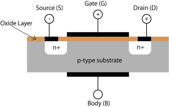
The way it's supposed to work is: When the transistor is off, no current flows. When it is on, current flows from the "Source" (the white region marked "n+" on the left) to the "Drain" (the white region marked "n+" on the right), along a thin layer underneath the "Oxide Layer" called the "Channel" or "Inversion Layer". No other current is supposed to flow within the transistor.
The way the current is allowed to pass through is by applying a positive voltage to the gate electrode, which creates an electric field across the oxide layer. This field repels holes (positive charges) and attracts electrons in the region marked "p-type substrate", with the result of forming an electron-conducting channel between the source and the drain. Ideally, the current through this channel is supposed to start flowing precisely when the voltage on the gate electrode reaches the value , for threshold voltage.
(Note that the kind of MOS transistor shown above is an "nMOS"; current integrated circuits combine nMOS with "pMOS" transistors, which are essentially the complement of nMOS in terms of positive and negative charges/p-type and n-type doping. This technology combining nMOS and pMOS transistors is known as "CMOS", where the C stands for Complementary.)
In reality, current leaks. Substhreshold leakage flows from the source to the drain when the voltage applied to the gate electrode is lower than the threshold voltage, i.e. when the transistor is supposed to be off. Gate oxide leakage flows from the gate electrode into the body (through the oxide layer). Junction leakage flows from the source and from the drain into the body (through the source-body and the drain-body junctions).
Gate oxide leakage and junction leakage are (mainly? entirely?) a matter of charges tunnelling through the ever thinner oxide layer or junction, respectively.
Subthreshold leakage does not depend on quantum effects and has been appreciable for much longer than the other two types of leakage, although it has only started to become unmanageable around 2004. It can be thought of as an issue of electrons spilling over the energy barrier formed by the (lightly doped) body-substrate between the (highly doped) source and drain regions. The higher the temperature of the device, the higher the energy distribution of the electrons; so even if the energy barrier is higher than the average energy of the electrons, those electrons in the upper tail of the distribution will spill over.
The height of this energy barrier is closely related to the threshold voltage, and so the amount of leakage current depends heavily on this voltage, increasing by about a factor of 10 each time the threshold voltage drops by another 100 mV. Increasing the threshold voltage thus reduces leakage power, but it also makes the gates slower, because the number of electrons that can flow through the channel is roughly proportional to the difference between supply voltage and threshold voltage.
Historically, threshold voltages were so high that it was possible to scale the supply voltage, the threshold voltage, and the channel length together without subthreshold leakage becoming an issue. This concurrent scaling of supply power and linear dimensions is an essential aspect of Dennard scaling, which historically permitted to increase the number and speed of transistors exponentially without increasing overall energy consumption. But eventually the leakage started affecting overall chip power. For this reason, the threshold voltage and hence the supply voltage could no longer be scaled down as previously. Since, however, the power it takes to switch a gate is the product of the switched capacitance and the square of the supply voltage, and the overall power dissipation is the product of this with the clock frequency, something had to give as the supply voltage no longer scaled as previously. This issue now severely limits the potential to further increase the clock frequency.
Gate oxide leakage, from what I understand, also has a direct impact on transistor performance, as the current from source to drain is related to the capacitance of the gate oxide, which is related to its area and inversely related to its thickness. Historically, the reduction in thickness compensated for the reduction in area as the device was scaled down in every generation, allowing to maintain and even improve the performance. As further reductions of the gate oxide thickness have become impossible due to excessive tunnelling, the industry has resorted to using higher-k materials for the gate oxide, i.e. material with a higher dielectric constant , as an alternative way of increasing the gate oxide capacitance (k and
are often used interchangeably in this context). However, recent roadmaps state that the success of this approach is already proving insufficient.
Overall, I believe it is pertinent to say that all kinds of leakage negatively affect performance by simply reducing the available usable power and by causing excessive heat dissipation, placing higher demands on packaging.
Two (gated) papers that describe these leakage issues in more detail (and there is a lot more detail to it) can be found here and here.
(cont'd)
(cont'd from previous comment)
Did the industry predict these problems and their consequences?
People in the industry were well aware of these limitations, long before they actually became critical. However, whether solutions and workarounds would be found was a matter of much greater uncertainty.
Robert Dennard et al's seminal 1974 paper Design of Ion-Implanted MOSFETs with Very Small Physical Dimensions, that described the very favourable scaling properties of MOSFET transistors and gave rise to the term "Dennard scaling", explicitly mentions the scaling limitations posed by subthreshold leakage:
One area in which the device characteristics fail to scale is in the subthreshold or weak inversion region of the turn-on characteristic. (…) In order to design devices for operation at room temperature and above, one must accept the fact that the subthreshold behavior does not scale as desired. This nonscaling property of the subthreshold characteristic is of particular concern to miniature dynamic memory circuits which require low source-to-drain leakage currents.
This influential 1995 paper by Davari, Dennard and Shahidi presents guidelines for transistor scaling for the years up to 2004. This paper contains a subsection titled "Performance/Power Tradeoff and Nonscalability of the Threshold Voltage", which explains the problems described above in a lot more detail than I have. The paper also mentions tunnelling through the gate oxide layer, concluding on both issues that they would remain relatively unproblematic up until 2004.
Subthreshold leakage is textbook material. The main textbook I have consulted is Digital Integrated Circuits by Jan Rabaey, and I have compared some aspects of the 1995 and 2003 editions. Both contained this sentence in the "History of…" chapter:
Interestingly enough, power consumption concerns are rapidly becoming dominant in CMOS design as well, and this time there does not seem to be a new technology around the corner to alleviate the problem.
Regarding gate oxide leakage, this comparatively very accessible 2007 article from the IEEE spectrum recounts the story of how engineers at Intel and elsewhere have developed transistors that use high- dielectrics as a way of maintaining the shrinking gate oxide's capacitance even as its thickness would cease to be reduced to prevent excessive tunnelling. According to this article, work on such solutions began in the mid-1990s, and Intel eventually launched new chips that made use of this technology in 2007. The main impression this article leaves me with is that the problem was very easy to foresee, but that finding out which solutions might work was a matter of extensive tinkering with highly unpredictable results.
The leakage issues are all mentioned in 2001 ITRS roadmap, the earliest edition that is available online. One example from the Executive Summary:
For low power logic (mainly for portable applications), the main issue is low leakage current, which is absolutely necessary in order to extend battery life. Device performance is then maximized according to the low leakage current requirements. Gate leakage current must be controlled, as well as sub-threshold leakage and junction leakage, including band-to-band tunneling. Preliminary analysis indicates that, balancing the gate leakage control requirements against performance requirements, high
may be required for the gate dielectric by around the year 2005.
From reading the reports, it is hard to make out whether the implications of these issues were correctly understood, and I have had to draw on a lot of other literature to get a better sense of where the industry stood on this. Getting a hold of earlier editions (the 1999 one in particular) and talking to industry insiders might shed a lot more light on the weight that was given to the different issues that were flagged as part of the "Red Brick Wall" I've mentioned above, i.e. as issues that had no known manufacturable solutions (I did not receive an answer to my inquiry about this from the contact person at the ITRS website). The Executive Summary of the 2001 edition states:
The 1999 ITRS warned that there was a wide range of solutions needed but unavailable to meet the technology requirements corresponding to 100 nm technology node. The 1999 ITRS edition also reported the presence of a potential “Red Brick Wall” or “100 nm Wall” (as indicated by the red cells in the technology requirements) that, by 2005, could block further scaling as predicted by Moore’s Law. However, technological progress continues to accelerate. In the process of compiling information for 2001 ITRS, it was clarified that this “Red Brick Wall” could be reached as early as 2003.
Two accessible articles from 2000 give a clearer impression of how this Red Brick Wall was perceived in the industry at the time. Both particularly emphasise gate oxide leakage.
(cont'd)
(cont'd from previous comment)
As I have mentioned at the beginning, the reports up to 2005 contained highly overoptimistic projections for on-chip frequency and supply voltage, which became dramatically more pessimistic in the 2007 edition. The reports clearly state, however, that these numbers are meant as targets and are not necessarily "on the road to sure implementation", especially where it has been highlighted that solutions were needed and not yet known. They can therefore not necessarily serve as a clear indictment of the ITRS' predictive powers, but I remain puzzled by some of their projections and comments on these before 2007. Getting clarification on this from industry insiders was the next thing I had planned for this project before we paused it.
Specifically, tables 4c and 4d in the Overall Roadmap Technology Characteristics, found in a subsection of the Executive Summary titled Performance of Packaged Chips, contain on-chip frequency forecasts in MHz, which became dramatically more pessimistic in 2007 than they had been in the previous 3 editions. A footnote in the 2007 edition states:
after 2007, the PIDS model fundamental reduction rate of ~ -14.7% for the transistor delay results in an individual transistor frequency performance rate increase of ~17.2% per year growth. In the 2005 roadmap, the trend of the on-chip frequency was also increased at the same rate of the maximum transistor performance through 2022. Although the 17% transistor performance trend target is continued in the PIDS TWG outlook, the Design TWG has revised the long-range on-chip frequency trend to be only about 8% growth rate per year. This is to reflect recent on-chip frequency slowing trends and anticipated speed-power design tradeoffs to manage a maximum 200 watts/chip affordable power management tradeoff.
Later editions seem to have reduced the expected scaling factor even further (1.04 in the 2011 edition), but there were also changes made to the metric employed, so I am not sure how to interpret the numbers (though I would expect the scaling factor to be unaffected by those changes).
Relatedly, a paragraph in the System Drivers document titled Maximum on-chip (global) clock frequency states that the on-chip clock frequency would not continue scaling at a factor of 2 per generation for several reasons. The 2001 edition states 3 reasons for this, the 2003 and 2005 edition state 4. But only in 2007 was the limitation from maximum allowable power dissipation added to this list of reasons. This strikes me as very puzzling. The paragraph, as it appears in the 2007 edition, is (emphasis added):
Maximum on-chip (global) clock frequency—(...) Through the 2000 ITRS, the MPU maximum on-chip clock frequency was modeled to increase by a factor of 2 per generation. Of this, approximately 1.4× was historically realized by device scaling (17%/year improvement in CV/I metric); the other 1.4× was obtained by reduction in number of logic stages in a pipeline stage (e.g., equivalent of 32 fanout-of-4 inverter (FO4 INV) delays13 at 180 nm, going to 24–26 FO4 INV delays at 130 nm). As noted in the 2001 ITRS, there are several reasons why this historical trend could not continue: 1) well-formed clock pulses cannot be generated with period below 6–8 FO4 INV delays; 2) there is increased overhead (diminishing returns) in pipelining (2–3 FO4 INV delays per flip-flop, 1–1.5 FO4 INV delays per pulse-mode latch); 3) thermal envelopes imposed by affordable packaging discourage very deep pipelining, and 4) architectural and circuit innovations increasingly defer the impact of worsening interconnect RCs (relative to devices) rather than contribute directly to frequency improvements. Recent editions of the ITRS flattened the MPU clock period at 12 FO4 INV delays at 90 nm (a plot of historical MPU clock period data is provided online at public.itrs.net), so that clock frequencies advanced only with device performance in the absence of novel circuit and architectural approaches. In 2007, we recognize the additional limitation from maximum allowable power dissipation. Modern MPU platforms have stabilized maximum power dissipation at approximately 120W due to package cost, reliability, and cooling cost issues. With a flat power requirement, the updated MPU clock frequency model starts with 4.7 GHz in 2007 and is projected to increase by a factor of at most 1.25× per technology generation, despite aggressive development and deployment of low-power design techniques.
Finally, the Overall Roadmap Technology Characteristics tables 6a and 6b (found in a subsection titled Power Supply and Power Dissipation in the Executive Summary) contains projected values of the supply power () which also became dramatically more pessimistic in the 2007 edition.
I have indicated my puzzlement at these points in an email I have sent out to a number of industry insiders, then asking:
Do the 3 revisions made to the roadmap in 2007 that I've pointed out reflect a failure of previous editions to predict the "breakdown in the serial speed version of Moore's Law" and the relevant issues that would cause it? Or do they merely reflect the ambitiousness and aggressiveness of the targets that were set before admitting defeat became inevitable?
I have received some very kind replies to those emails, but most have focused on the technical reasons for the "breakdown" in Dennard scaling. The only comment I have received on this last question was from Robert Dennard, who sent me a particularly thoughtful email that came with 4 attachments (which mainly provided more technical detail on transistor design, however). At the end of his email, he wrote:
I cannot comment on wishful thinking vs hard facts. Predicting the future is difficult. Betting against Moore's Law was often a losing game. Texas Instruments quit way to early.
Indeed, which bets it is most rational to make depends on expected payoff ratios as well as on probability estimates. This distinction between targets and mere predictions complicates the question quite a bit.
This was an interesting project, it would be great to pick it up again.
(cont'd from previous comment)
Did the industry predict these problems and their consequences?
People in the industry were well aware of these limitations, long before they actually became critical. However, whether solutions and workarounds would be found was a matter of much greater uncertainty.
Robert Dennard et al's seminal 1974 paper Design of Ion-Implanted MOSFETs with Very Small Physical Dimensions, that described the very favourable scaling properties of MOSFET transistors and gave rise to the term "Dennard scaling", explicitly mentions the scaling limitations posed by subthreshold leakage:
One area in which the device characteristics fail to scale is in the subthreshold or weak inversion region of the turn-on characteristic. (…) In order to design devices for operation at room temperature and above, one must accept the fact that the subthreshold behavior does not scale as desired. This nonscaling property of the subthreshold characteristic is of particular concern to miniature dynamic memory circuits which require low source-to-drain leakage currents.
This influential 1995 paper by Davari, Dennard and Shahidi presents guidelines for transistor scaling for the years up to 2004. This paper contains a subsection titled "Performance/Power Tradeoff and Nonscalability of the Threshold Voltage", which explains the problems described above in a lot more detail than I have. The paper also mentions tunnelling through the gate oxide layer, concluding on both issues that they would remain relatively unproblematic up until 2004.
Subthreshold leakage is textbook material. The main textbook I have consulted is Digital Integrated Circuits by Jan Rabaey, and I have compared some aspects of the 1995 and 2003 editions. Both contained this sentence in the "History of…" chapter:
Interestingly enough, power consumption concerns are rapidly becoming dominant in CMOS design as well, and this time there does not seem to be a new technology around the corner to alleviate the problem.
Regarding gate oxide leakage, this comparatively very accessible 2007 article from the IEEE spectrum recounts the story of how engineers at Intel and elsewhere have developed transistors that use high- dielectrics as a way of maintaining the shrinking gate oxide's capacitance even as its thickness would cease to be reduced to prevent excessive tunnelling. According to this article, work on such solutions began in the mid-1990s, and Intel eventually launched new chips that made use of this technology in 2007. The main impression this article leaves me with is that the problem was very easy to foresee, but that finding out which solutions might work was a matter of extensive tinkering with highly unpredictable results.
The leakage issues are all mentioned in 2001 ITRS roadmap, the earliest edition that is available online. One example from the Executive Summary:
For low power logic (mainly for portable applications), the main issue is low leakage current, which is absolutely necessary in order to extend battery life. Device performance is then maximized according to the low leakage current requirements. Gate leakage current must be controlled, as well as sub-threshold leakage and junction leakage, including band-to-band tunneling. Preliminary analysis indicates that, balancing the gate leakage control requirements against performance requirements, high
From reading the reports, it is hard to make out whether the implications of these issues were correctly understood, and I have had to draw on a lot of other literature to get a better sense of where the industry stood on this. Getting a hold of earlier editions (the 1999 one in particular) and talking to industry insiders might shed a lot more light on the weight that was given to the different issues that were flagged as part of the "Red Brick Wall" I've mentioned above, i.e. as issues that had no known manufacturable solutions (I did not receive an answer to my inquiry about this from the contact person at the ITRS website). The Executive Summary of the 2001 edition states:
The 1999 ITRS warned that there was a wide range of solutions needed but unavailable to meet the technology requirements corresponding to 100 nm technology node. The 1999 ITRS edition also reported the presence of a potential “Red Brick Wall” or “100 nm Wall” (as indicated by the red cells in the technology requirements) that, by 2005, could block further scaling as predicted by Moore’s Law. However, technological progress continues to accelerate. In the process of compiling information for 2001 ITRS, it was clarified that this “Red Brick Wall” could be reached as early as 2003.
Two accessible articles from 2000 give a clearer impression of how this Red Brick Wall was perceived in the industry at the time. Both particularly emphasise gate oxide leakage.
(cont'd)
When IBM bottled out of going to 4 GHz CPUs, in 2004, they had a roadmap extending to at least 5. Maybe beyond, I don't remember, but certainly there was general loose talk in the trade rags about 10 or 20 GHz in the foreseeable.
2: An outside view works best when using a reference class with a similar causal structure to the thing you're trying to predict. An inside view works best when a phenomenon's causal structure is well-understood, and when (to your knowledge) there are very few phenomena with a similar causal structure that you can use to predict things about the phenomenon you're investigating. See: The Outside View's Domain.
When writing a textbook that's much like other textbooks, you're probably best off predicting the cost and duration of the project by looking at similar textbook-writing projects. When you're predicting the trajectory of the serial speed formulation of Moore's Law, or predicting which spaceship designs will successfully land humans on the moon for the first time, you're probably best off using an (intensely informed) inside view.
Is there data/experiments on when each gives better predictions, as with Kahneman's original outside view work?
Doesn't the act of combining many outside views and their reference classes turn you into somebody operating on the inside view? This is to say, what is the difference between this and the type of "inside" reasoning about a phenomenon's causal structure?
Is it that inside thinking involves the construction of new models whereas outside thinking involves comparison and combination of existing models? From an machine intelligence perspective, the distinction is meaningless. The construction of new models is the extension of old models, albeit models of arbitrary simplicity. Deductive reasoning is just the generation of some new strings for induction to operate on to generate probabilities. Induction has the final word; that's where the Bayesian network is queried for the result. Logic is the intentional generation of reference classes, a strategy for generating experiments that are likely to quickly converge that probability to 0 or 1.
Inside thinking also, analogously in humans, is the generation of new reference classes; after casting the spell called Reason, the phenomenon now belongs to a class of referents that upon doing so produce a particularly distinguishing set of strings in my brain. The existence of these strings, for the outside thinker, is strong evidence about the nature of the phenomenon. And once the strings exist, the outside thinker is required to combine the model that includes them with her existing model. And unbeknownst to the outside thinker, the strategy of seeking new reference classes is inside thinking.
Doesn't the act of combining many outside views and their reference classes turn you into somebody operating on the inside view?
Yes. So does the act of selecting just one outside view as your Personal Favorite, since it gives the right answer.
I think that's only true if you allow yourself free choice of outside views. If you had a fixed frameworks of which outside views to take into account, i.e. how to select the ten experts you're going to ask for their opinion, and you decide that before you formulate the problem, the composite model you get shouldn't suffer from the arbitrariness of the inside view. Right?
It looks like the different views are the predictions of models learned on different time scales. The outside view has a small learning rate, so it reflects the long time-scale features of your observation history (or your species' history, if you're using evolved intuitions) and habitual control policies. The inside view is forgetful, so it updates its beliefs a lot in response to recent evidence, and is more likely to diverge or oscillate than converge to true beliefs or low cost trajectories, relative to the outside view. This perspective doesn't explain why the inside view would be systemically optimistic.
I haven't had much explicit interaction with these inside/outside view concepts, and maybe I'm misunderstanding the terminology, but a couple of the examples of outside views given struck me as more like inside views: Yelp reviews and the advice of a friend are calibrated instruments being used to measure the performance of a restaurant, ie to build a model of its internal workings.
But then almost immediately, I thought, "hey, even the inside view is an outside view." Every model is an analogy, e.g. an analogy in the sense of this thing A is a bit like thing B, so probably it will behave analogously, or e.g. 5 seconds ago the thing in my pocket was my wallet, so the thing in my pocket is probably still my wallet. It doesn't really matter if the symmetry we exploit in our modeling involves translation through space, translation from one bit of matter to another, or translation through time: strictly speaking, it's still an analogy.
I have no strong idea what implications this might have for problem solving. Perhaps there is another way of refining the language that helps. What I'm inclined to identify as the salient features of (what I understand to be) the inside view is that (subject to some super-model) there is a reasonable probability that the chosen model is correct, whereas for the outside view we are fairly certain that the chosen model is not correct, though it may still be useful. This strikes me as usefully linked to the excellent suggestions here regarding weighted application of multiple models. Perhaps the distinction between inside and outside views is a red herring, and we should concentrate instead on working out our confidence in each available model's ability to provide useful predictions, acknowledging that all models are necessarily founded on analogies, with differing degrees of relevance.
Keynes in his "Treatise on probability" talks a lot about analogies in the sense you use it here, particularly in "part 3: induction and analogy". You might find it interesting.
I only know two outside views that result in projections of time to AI, which are (1) looking at AI as a specific technology like Kurzweil or Nagy, and (2) AI as a civilizational transition like Hanson. Of these, I've recently decided I prefer Hanson's approach because it seems to match the scale of the transition better, and it seems misguided to view machines that beat humans at all capabilities as one specific technology anyway as opposed to a confluence of hardware and various software things (or brain scanning if you're an ems fan).
A problem with Kurzweil's approach is that modern computer growth trends only started--according to William Nordhaus anyway--around 1940. So who is to say this thing could not just shut off? Indeed, if you take it as one of the performance curves analyzed by Nagy, then maybe as an unusually long-lasting trend it has a higher chance of stopping than if you naively said, "Moore's Law has lasted 70 years, so there's a 50/50 chance of it lasting 70 more years."
Ideally a pretty good way to go, making use of your suggestion of model combination, might be to let Hanson's reasoning about GDP doubling times form 3/4 of your probability distribution, and then somehow splice in 1/4 based on specific trends happening now--although not just hardware. But that last requirement means I in practice don't know how to do this.
If anybody thinks they have done better I'd really like to hear about it.
In mathematical terms, the map from problem space to reference classes is a projection and has no canonical choice (you apply the projection by choosing to lose information), whereas the map from causal structures to problem space is an imbedding and has such a choice (and the choice gains information).
I suspect the key distinction may the difference between extrapolation and interpolation. The outside view is far and away more reliable for interpolation: i.e. we have many events on both sides of the one we're attempting to model. Extrapolation, where we have data only on one side of the event we're trying to model, runs a much greater risk of failing in the outside view. The risk of failing in the inside view is no less in this case than with interpolation, but in this case the outside view is not as strong a predictor.
When writing a textbook that's much like other textbooks, you're probably best off predicting the cost and duration of the project by looking at similar textbook-writing projects.
http://www.mckinsey.com/insights/strategy/daniel_kahneman_beware_the_inside_view
did I gwern in?
If the difference is between inference from surface features vs. internal structure, then yes of course in either case unless you have a very strong theory, you will probably do better to combine many weak theories. When looking at surface features, look at many different features, not just one.
Inside and outside views: a quick review
1. There are two ways you might predict outcomes for a phenomenon. If you make your predictions using a detailed visualization of how something works, you're using an inside view. If instead you ignore the details of how something works, and instead make your predictions by assuming that a phenomenon will behave roughly like other similar phenomena, you're using an outside view (also called reference class forecasting).
Inside view examples:
Outside view examples:
See also chapter 23 in Kahneman (2011); Planning Fallacy; Reference class forecasting. Note that, after several decades of past success, the serial speed formulation of Moore's Law did in fact break down in 2004 for the reasons described (Fuller & Millett 2011).
2. An outside view works best when using a reference class with a similar causal structure to the thing you're trying to predict. An inside view works best when a phenomenon's causal structure is well-understood, and when (to your knowledge) there are very few phenomena with a similar causal structure that you can use to predict things about the phenomenon you're investigating. See: The Outside View's Domain.
When writing a textbook that's much like other textbooks, you're probably best off predicting the cost and duration of the project by looking at similar textbook-writing projects. When you're predicting the trajectory of the serial speed formulation of Moore's Law, or predicting which spaceship designs will successfully land humans on the moon for the first time, you're probably best off using an (intensely informed) inside view.
3. Some things aren't very predictable with either an outside view or an inside view. Sometimes, the thing you're trying to predict seems to have a significantly different causal structure than other things, and you don't understand its causal structure very well. What should we do in such cases? This remains a matter of debate.
Eliezer Yudkowsky recommends a weak inside view for such cases:
In contrast, Robin Hanson recommends an outside view for difficult cases:
In Yudkowsky (2013), sec. 2.1, Yudkowsky offers a reply to these paragraphs, and continues to advocate for a weak inside view. He also adds:
This is the problem of "reference class tennis": each participant in the debate claims their own reference class is most appropriate for predicting the phenomenon under discussion, and if disagreement remains, they might each say "I’m taking my reference class and going home."
Responding to the same point made elsewhere, Robin Hanson wrote:
Multiple reference classes
Yudkowsky (2013) adds one more complaint about reference class forecasting in difficult forecasting circumstances:
Both this comment and Hanson's last comment above point to the vulnerability of relying on any single reference class, at least for difficult forecasting problems. Beware brittle arguments, says Paul Christiano.
One obvious solution is to use multiple reference classes, and weight them by how relevant you think they are to the phenomenon you're trying to predict. Holden Karnofsky writes of investigating things from "many different angles." Jonah Sinick refers to "many weak arguments." Statisticians call this "model combination." Machine learning researchers call it "ensemble learning" or "classifier combination."
In other words, we can use many outside views.
Nate Silver does this when he predicts elections (see Silver 2012, ch. 2). Venture capitalists do this when they evaluate startups. The best political forecasters studied in Tetlock (2005), the "foxes," tended to do this.
In fact, most of us do this regularly.
How do you predict which restaurant's food you'll most enjoy, when visiting San Francisco for the first time? One outside view comes from the restaurant's Yelp reviews. Another outside view comes from your friend Jade's opinion. Another outside view comes from the fact that you usually enjoy Asian cuisines more than other cuisines. And so on. Then you combine these different models of the situation, weighting them by how robustly they each tend to predict your eating enjoyment, and you grab a taxi to Osha Thai.
(Technical note: I say "model combination" rather than "model averaging" on purpose.)
Model combination and adjustment
You can probably do even better than this, though — if you know some things about the phenomenon and you're very careful. Once you've combined a handful of models to arrive at a qualitative or quantitative judgment, you should still be able to "adjust" the judgment in some cases using an inside view.
For example, suppose I used the above process, and I plan to visit Osha Thai for dinner. Then, somebody gives me my first taste of the Synsepalum dulcificum fruit. I happen to know that this fruit contains a molecule called miraculin which binds to one's tastebuds and makes sour foods taste sweet, and that this effect lasts for about an hour (Koizumi et al. 2011). Despite the results of my earlier model combination, I predict I won't particularly enjoy Osha Thai at the moment. Instead, I decide to try some tabasco sauce, to see whether it now tastes like doughnut glaze.
In some cases, you might also need to adjust for your prior over, say, "expected enjoyment of restaurant food," if for some reason your original model combination procedure didn't capture your prior properly.
Against "the outside view"
There is a lot more to say about model combination and adjustment (e.g. this), but for now let me make a suggestion about language usage.
Sometimes, small changes to our language can help us think more accurately. For example, gender-neutral language can reduce male bias in our associations (Stahlberg et al. 2007). In this spirit, I recommend we retire the phrase "the outside view..", and instead use phrases like "some outside views..." and "an outside view..."
My reasons are:
Speaking of "the" outside view privileges a particular reference class, which could make us overconfident of that particular model's predictions, and leave model uncertainty unaccounted for.
Speaking of "the" outside view can act as a conversation-stopper, whereas speaking of multiple outside views encourages further discussion about how much weight each model should be given, and what each of them implies about the phenomenon under discussion.