This is a series of snippets about the Google DeepMind mechanistic interpretability team's research into Sparse Autoencoders, that didn't meet our bar for a full paper. Please start at the summary post for more context, and a summary of each snippet. They can be read in any order.

Activation Steering with SAEs

Arthur Conmy, Neel Nanda

TL;DR: We use SAEs trained on GPT-2 XL’s residual stream to decompose steering vectors into interpretable features. We find a single SAE feature for anger which is a Pareto-improvement over the anger steering vector from existing work (Section 3, 3 minute read). We have more mixed results with wedding steering vectors: we can partially interpret the vectors, but the SAE reconstruction is a slightly worse steering vector, and just taking the obvious features produces a notably worse vector. We can produce a better steering vector by removing SAE features which are irrelevant (Section 4). This is one of the first examples of SAEs having any success for enabling better control of language models, and we are excited to continue exploring this in future work. 

1. Background and Motivation

We are uncertain about how useful mechanistic interpretability research, including SAE research, will be for AI safety and alignment. Unlike RLHF and dangerous capability evaluation (for example), mechanistic interpretability is not currently very useful for downstream applications on models. Though there are ambitious goals for mechanistic interpretability research such as finding safety-relevant features in language models using SAEs, these are likely not tractable on the relatively small base models we study in all our snippets.

To address these two concerns, we decided to study activation steering^[1] (introduced in this blog post and expanded on in a paper). We recommend skimming the blog post for an explanation of the technique and examples of what it can do. Briefly, activation steering takes vector(s) from the residual stream on some prompt(s), and then adds these to the residual stream on a second prompt. This makes outputs from the second forward pass have properties inherited from the first forward pass. There is early evidence that this technique could help with safety-relevant properties of LLMs, such as sycophancy.

We have tentative early research results that suggest SAEs are helpful for improving and interpreting steering vectors, albeit with limitations. We find these results particularly exciting as they provide evidence that SAEs can identify causally meaningful intermediate variables in the model, indicating that they aren’t just finding clusters in the data or directions in logit space, which seemed much more likely before we did this research. We plan to continue this research to further validate SAEs and to gain more intuition about what features SAEs do and don’t learn in practice.

2. Setup

We use SAEs trained on the residual stream of GPT-2 XL at various layers, the model used in the initial activation steering blog post, inspired by the success of residual stream SAEs on GPT-2 Small (Bloom, 2024) and Pythia models (Cunningham et. al, 2023). The SAEs have 131072 learned features, L0 of around 60^[2], and loss recovered around 97.5% (e.g. splicing in the SAE from Section 3 increases loss from 2.88 to 3.06, compared to the destructive zero ablation intervention resulting in Loss > 10). We don’t think this was a particularly high-quality SAE, as the majority of its learned features were dead, and we found limitations with training residual stream SAEs that we will discuss in an upcoming paper. Even despite this, we think the results in this work are tentative evidence for SAEs being useful. 

It is likely easiest to simply read our results in Section 3, but our full methodology is as follows: 

To evaluate how effective different steering vectors are, we look at two metrics: 

1. The proportion of rollouts that contain vocabulary from a certain target vocabulary (e.g. wedding-related words)^[3] - i.e., did we successfully steer the model? We call this P(Successful Rollout)
2. The average cross-entropy loss of the model on pretraining data when we add the steering vector while computing the forward pass^[4]. i.e., did we break the model?^[5] We call this the Spliced LLM Loss. 

We then vary the coefficient of the steering vector added and look at the Pareto frontier for different methods of adding activation vectors. We didn’t find any directly applicable comparison to the original steering vector post, so chose this simple-to-compute metric. The methods we compared were:

1. Original steering vectors: we use the exact method described in the original steering vector post to obtain steering vectors for a baseline.
2. SAE reconstructions: In all experiments where we use SAEs, we take original steering vectors and pass them through the Sparse Autoencoder to obtain a reconstruction as a sparse sum of learned features (we use the reconstruction for different purposes, as described below).

In both cases, we use the same sampling hyperparameters as the original blog post.

3. Improving the “Anger” Steering Vector

In the initial activation steering blog post the authors inject the difference between activations on “|BOS|An|ger|'' and “|BOS|Ca|lm|'' before Layer 20 in the residual stream into prompts beginning “|BOS|I| think| you|'re|” to steer the model towards angry completions (see Footnote 11). 

Using an SAE trained on L20 residual stream states, we look at the active features on the “ger” token of the “|BOS|An|ger|'' input. 

We find that the feature that fires most, contributing 16% of the L1 score (summed feature activations) on this token, is clearly identifying anger through its direct logit attribution and max activating examples:

Excitingly, we find that simply adding this anger feature vector (with the same coefficient) at the “| think|” token in “|BOS|I| think| you|'re|” is more effective than the methodology from the original activation steering post, despite being just one component of the vector they used!

An important hyper-parameter when steering is the coefficient of the steering vector when it’s added to the residual stream. Larger coefficients^[6] tend to have more effect (until a certain point) but also worsen model performance more. To visualise our results we plot the frontier for a given vector against the P(Successful Rollout)^[7] and Spliced LLM Loss metrics, and see that the anger feature is a Pareto improvement! 

 The rollouts for the steering vector with maximal anger-related word count seem coherent, by observing the first four:

• I think you're an idiot. You've been told that the law is the law, and that if you don't like it, you should just go to another country. You're not allowed to complain about your job or your life or how much… ✅ (“idiot” is anger-related vocab)
• I think you're a fool. You are a child, and your parents have done nothing wrong. You are a child, and your parents have done nothing wrong. Your parents will never understand what you've been through. You'll never understand… ❌ (no anger-related vocab detected, though this is likely a false negative)
• I think you're an idiot. I'm not sure why you would want to do this, but I'm going to do it anyway. The first thing that happened was that the package arrived at my house and I opened it up and found a letter inside with… ✅ (“idiot”)
• I think you're a stupid f****** c***. I'm going to go back to my room and start reading some books about the consequences of stupidity. The book is called "How To Be A Person" by David Foster Wallace, and it's a collection of essays… ✅ (“f*******”, “c***”)

These rollouts used just over 30x the magnitude of the feature in the SAE reconstruction (820.0).

4. Interpreting the “Wedding” Steering Vector

We tried to extend the success of SAE steering vectors to the “Weddings” example in the steering blog post, but found mixed results:

The SAE reconstruction has many interpretable features. 

Our first finding was generally positive: that SAEs were able to find a large number of interpretable features on these prompts, similarly to the experience in this work.  

The wedding steering vector is the difference between the activations on the prompt “|BOS|I| talk| about| weddings| constantly|” and “|BOS|I| do| not| talk| about| weddings| constantly|”. 

The largest positive activations of SAE features, taking into account cancellation from the “I do not talk about weddings” sentence^[9] were: 

• “ talk” position:
  • A “ talk” single-token feature of norm 56
• “ about” position:
  • An “ about” feature of norm 43
• “ weddings” position:
  • 63.1 norm “wedding(s)”/”weddings” feature.
  • A second “wedding(s)” feature (37 norm).
  • A 25 norm plurals feature.
  • One uninterpretable feature of norm 23.
  • A 14 norm |Wed|**dings**| feature.
  • There is also a 9.5 norm feature firing on tokens after a phrase like “talking about”.
• “ constantly” position:
  • A 31 norm “constantly” single token feature
  • A 18 norm “consistently/continually/routinely/etc” feature
  • A 14 norm “-ly” feature
  • A 13 norm feature firing on tokens after a phrase like “talking about” (but different from the feature on the “ weddings” token)
• Space token (for padding):
  • A 64 norm feature firing on spaces
  • A different, 19.8 norm feature firing on spaces
  • Also another, different 9.8 norm feature firing after ‘talking’/’speaking’

We find that almost all these vectors are interpretable once we ignore the dense features that fire on most tokens and that are almost cancelled by the activation steering method. However, notice that there seems to be a lot of feature splitting where several features encode really similar concepts. Also, the features are often extremely low level, which is likely less helpful for steering. 

Just using hand-picked interpretable features from the SAE led to a much worse steering vector.

Indeed, when we i) took the SAE’s sparse decomposition of the residual stream’s activations on the positive prompt (‘I talk about weddings constantly’), and then ii) removed all the features except the interpretable features from Section 2 above, and finally iii) scaled this resultant steering vector to produce a Pareto frontier, we see that the interpretable steering vector is Pareto dominated by the original steering vector^[10]:

The important SAE features for the wedding steer vector are less intuitive than the anger steering vector. 

Despite the failure of the naive method from 2., we found that it was still possible to use SAEs to obtain steering vectors (that were sadly not quite as effective as those from the original prompts). 

Instead of using the activations from the prompts “|BOS|I| talk| about| weddings| constantly|” and “|BOS|I| do| not| talk| about| weddings| constantly|”, we can pass both of these activations through the SAE in turn, and then take the difference of the SAE’s outputs (note that we do no further editing, e.g. we aren’t restricting to specific features in the SAE reconstruction, we’re just excluding the reconstruction error term from the SAE to verify that the SAEs aren’t losing the key info that makes the steering vector work).

The resulting Pareto frontier is notably worse for medium-sized norms of steering vectors, but slightly better for large or small norms of steering vectors. 

So, what was missing from our analysis in 2.? Removing as many unnecessary parts of our setup as possible, we narrowed down the important SAE features to: 

• The last three token positions, i.e. “...| weddings| constantly | |” and “...| about| weddings| constantly|” 
• The top (feature, position) pairs that occurred in at least one of: 1) the top 10 norm positive prompt features at a position or 2) the top 10 negative prompt features at a position^[11]. 

Surprisingly, we found that some of the features that strongly activated on the negative prompt’s final position were very important for the steering vector. Indeed, considering the baseline of only including (feature, position) pairs from the top 10 features activating on the positive prompt, we can improve the steering vector drastically by also including the top 3 or 5 features active on the negative prompt that are not active on the positive prompt. 

Looking at the first three features added, they appeared to correspond to interpretable directions on the subtracted “|constantly|” token, but we’re not sure why subtracting them led to a big difference in results. This could be both down to these features impacting the model in an unexpected way, or our Pareto frontier metric being limited. In future work, we hope to address these issues better. 

Removing interpretable but irrelevant SAE features from the original steering vector improves performance. 

Finally, we show an applications of SAEs to steering vectors that doesn’t depend on strong reconstructions. 

We also found that there are many unnecessary features, such as the space features, introduced solely due to padding input tokens to length (see 1.). We find that projecting out these two directions from the original vector (i.e. not the SAE reconstructed one) feature leads to better Pareto performance:

It also removes the double spaces (“| | |”) that can be found in the original subjective examples (we use a 2.0 multiplier, half the original blog post). The first four completions from this run: 

• I went up to my friend. I said, "How did you get into this?" He said, "I'm a writer." I said, "Oh, so you're a wedding planner?" He says, "No. I'm a wedding planner."
• I went up to my friend. "I'm not sure if you know this, but I'm a little bit of a big deal in the world of weddings."\n\n"Oh?" she said. "What do you mean?"\n\n"Well, I have been married…
• I went up to my friend, who is a bride and groom's photographer, and said "I want to take a picture of you on your wedding day." She was like "Oh that's so cool! I'm going to be wearing a white dress!"\n\nAnd I…
• I went up to my friend and asked her what she thought of the wedding. She said it was "awesome" and that she would be there. I was very excited, but then I realized that she had never been to a wedding before… 

Example failure case: 

• I went up to my friend. I said, "What's the deal with your hair?"\n\nHe said, "Oh, it's a mess."\n\n"How do you know?" I asked. He said he was a hairstylist and he had been cutting…

References

Activation Steering blog post.

Activation Steering paper.

This really helpful repo branch with the steering paper’s experiments.

LLAMA Activation Steering paper.

TransformerLens.

Callum’s SAE vis.

Residual stream SAEs: 1 and 2.

Bricken et al. 

Appendix

Please see this google doc for an appendix, with more feature dashboards, and pseudocode for generating steering vectors in TransformerLens.

Replacing SAE Encoders with Inference-Time Optimisation

Lewis Smith

TL;DR: The goal of SAEs is to find an interpretable, sparse reconstruction of activations. This involves two sub-problems: learning the dictionary of feature vectors (the decoder, $W_{dec}$ and computing the sparse coefficient vector on a given input (the encoder, a linear map followed by a ReLU). SAEs encourage us to think of these as two entangled subproblems, but they can be usefully separated. Here, we investigate using ‘inference-time optimisation’ (ITO), where we take the dictionary of a trained SAE, throw away the encoder, and learn the sparse feature coefficients at inference time. We mainly use this as a way of studying the quality of the learned dictionary independent of how well the encoder works, though there are other potential applications we discuss briefly.

We describe a (known) algorithm to do ITO - gradient pursuit^[12] - which can approximately solve the sparse approximation problem^[13] and is amenable to implementation on accelerators. We also discuss some other interesting results we got by using inference time optimisation on dictionaries learned using sparse autoencoders, notably finding that training SAEs with high L0 creates higher quality dictionaries than lower L0 SAEs, even if we learn coefficients at low L0 at inference time.

Inference Time Optimisation

The dictionary learning problem we are solving with SAEs can be thought of as two separate problems. Sparse coding tries to learn an appropriate sparse dictionary from data. Sparse approximation tries to find the best reconstruction of a given signal using a sparse combination of a fixed dictionary of vectors. Naturally, these problems are highly related: sparse coding methods often have to solve a sparse approximation problem in an inner loop, and sparse approximation requires a dictionary, often produced by sparse coding. We want to use sparse coding to recover the dictionary of underlying feature directions used by the model, and sparse approximation to decompose a given activation vector into a (sparse) weighted sum of these feature directions.

SAEs combine learning a dictionary (the decoder weights) and a sparse approximation algorithm (the encoder - a linear map followed by a ReLU) into a single neural network, so it’s natural to think of it as a single unit. Further, both the encoder and decoder are parameterized by a matrix of weights from $d_{model}$ to $d_{sae}$ or back, so it’s natural to think of them as somehow “symmetric” operations. However, these are logically separate steps. We’ve found this a useful conceptual clarification for reasoning about SAEs.  

The decoder we have learnt training our SAE is just a sparse dictionary, so we can in principle use any sparse approximation algorithm to reconstruct a signal using it. We refer to this as inference-time optimisation: taking a dictionary of a trained SAE, and learning coefficients for it for a given activation at inference time.

There are a few potential reasons that non-SAE sparse approximation methods could be interesting for interpretability, but our primary motivation in this snippet is that it lets us separate the evaluation of the sparse coding from our evaluation of the sparse approximation that our SAEs are doing, as we can evaluate two different sparse dictionaries using the same sparse approximation algorithm to study the quality of the dictionary independently of the encoder. For some downstream applications - such as our experiments on steering vectors - we only care about the feature directions learnt, and so it would be useful to have a principled way to evaluate the codebook quality in isolation. For instance, later in this snippet we describe results that suggest that training SAEs with a higher L0 may result in better dictionaries, even if you want to use a sparser reconstruction at test time.

Another reason we might be interested in using more powerful sparse approximation algorithms at test time is that this could improve the quality of our reconstruction. Standard SAEs are prone to issues like shrinkage which reduce the quality of reconstruction (see, for example, this work), and we certainly find that we can increase the loss recovered when patching in the SAE by using a more powerful sparse approximation algorithm instead of the encoder. Whether these reconstructions are as interpretable as those chosen by a linear encoder remains an open question, though we do provide some early analysis in this snippet. 

In theory, we could also replace SAEs entirely, and use a more classical sparse coding algorithm to learn the dictionary as well. We do not study this in this snippet. In Anthropic's work on dictionary learning, they choose a sparse autoencoder rather than powerful dictionary learning methods because they are worried that using a more powerful sparse approximation algorithm to learn the dictionary might find ‘features’ which the neural network does not actually use, partly because it seems implausible that the network can be using an iterative sparse approximation algorithm to recover features from superposition. We think this is an important concern. Our goal is not just to find a sparse reconstruction, it’s to find the (hopefully interpretable) features that the model actually uses, but it’s both hard to measure this and to optimize explicitly for it. We focus on inference-time optimisation specifically in this snippet because we think it’s much less vulnerable to this concern, as we use a dictionary learnt using a sparse autoencoder. On the other hand, if we are happy that inference time optimisation gives us interpretable reconstructions, then experimenting with using more classical sparse coding techniques which use iterative sparse approximation as a subroutine would be a natural thing to experiment with. Part of the reason that we have not experimented with this yet is that, currently, we think that we lack really good methods for comparing one SAE to another apart from manual analysis, which is time consuming and difficult. However, as we develop tools like autointerp, automatic circuit analysis and steering which let us evaluate sparse codes more objectively, we think that experimenting more with methods like this could be an interesting possible future direction. 

Empirical Results 

Inference time optimisation gives us a way to compare the quality of a learned dictionary independently of both the encoder and the target sparsity level, as we can hold the dictionary fixed and sweep the target sparsity of the reconstruction algorithm. This allows us to think about the optimal sparsity penalty (i.e the SAE L1 weight) for learning a dictionary, independently of the actual sparsity we want at test time. 

The graph below shows the pareto frontier for a set of SAE dictionaries trained with different L1 penalties on the post-activation site on a 1 layer model, when we apply inference-time optimisation. In the legend we've marked the L0 achieved by these dictionaries when used with their original SAE, the x-axis is the target L0 of the inference-time optimisation algorithm, and the y-axis shows the loss recovered. As we can see, the dictionary derived from the L0=99 SAE seems to have the best Pareto curve, even beating dictionaries trained with lower L0 at low L0s.

We also show in gray the pareto curve formed by the loss recovered of using the original encoder with their corresponding dictionary, demonstrating that applying ITO generally leads to a significant improvement in loss recovered at a given sparsity level (as we would expect given that it’s a more powerful algorithm than a linear encoder). Note that each point in the ‘encoder’ curve is a different dictionary, whereas using ITO we can sweep the target L0 for each dictionary. We also plot using ITO with a randomly chosen dictionary of the same size as the SAE decoder as a baseline, finding that this performs very poorly.

We see similar results for different sites and larger models.

We find this result striking, as it suggests we should perhaps be training SAEs at a higher L0 than seems optimal for interpretability, and then reducing the L0 post-hoc (e.g. via ITO, or by simpler interventions like just taking the top k coefficients), as the dictionaries learnt by higher L0 SAEs seem to be pareto improvements over those learnt by very sparse models. 

We manually inspected a few features using ITO at inference time, and found no obvious difference in the interpretability of activations produced by either method.

However, there are significant differences, particularly in lower activating examples; ITO typically chooses different features than the SAE encoder as well as choosing the activation level differently, especially for lower activating features.

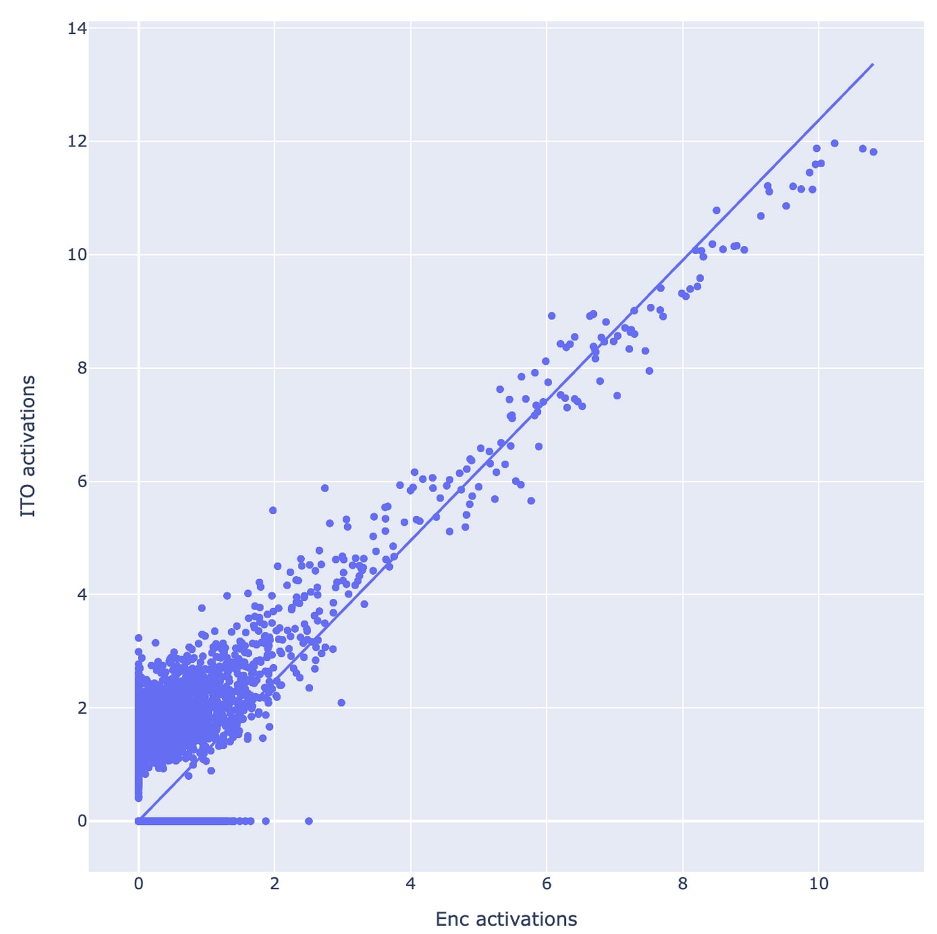
This is clear in the following graph, which shows the correlation between the activation for a feature predicted by ITO against the activation predicted by the learnt encoder for a particular SAE and an arbitrarily chosen feature (though we did check manually that the feature was interpretable). The chosen SAE has an l0 of around 40, and so we set the ITO to have this target sparsity as well. The figure shows that both methods tend to predict highly correlated activations when the feature is strongly present, but that low level activations are barely correlated. We’re not sure if low activations are mostly uninterpretable noise (where it may not be that surprising that they differ), or if this suggests something about how the two methods detect weak but real feature activations differently (or something else entirely!).

We note that these results may be somewhat biased. SAEs often have many small non-zero activations which aren’t very important for reconstruction or loss recovered but inflate the L0, probably due to the limitations of a linear encoder,  while gradient pursuit often has a far larger value for the smallest non-zero activation. This effect is also visible in the activation scatter plot; note that the ‘blob’ has a non-zero intercept with the y axis, showing that if gradient pursuit activates a feature, it tends to activate it strongly. 

Our current sense is that ITO is an interesting direction for future work, and at the very least can serve as a potentially valuable way to compare dictionary quality without depending on the encoder. We think there are likely ways to do this by building on the results here.

Another possible application is actually replacing the encoder at test time, to increase the loss recovered of the sparse decomposition. We don’t think we can justify advising using it as a drop in replacement for SAE encoders without a more detailed study of its interpretability compared to SAE encoders, but we think this is a potentially valuable future direction. 

Using algorithms similar to the one discussed here as a part of a sparse dictionary learning method as an alternative to SAEs could also be an interesting direction for future work, if the previous two seem promising.

Details of Sparse Approximation Algorithms (for accelerators)

This section gets into the technical weeds, and is intended to act as a guide to people who want to implement ITO for themselves on GPUs/TPUs using the specific algorithm we used.

The problem of sparse approximation with a fixed dictionary is well studied. While solving it optimally is NP-hard, there are many approximation algorithms which work well in practice. We have focused on the family of ‘matched pursuit’ algorithms. The central idea of matched pursuit is to choose the dictionary elements greedily. We choose the dictionary element with the largest inner product with the residual, subtract this vector from the residual so the residual is orthogonal to it, and iterate until the desired number of sparse vectors is reached. In pseudocode;

def matched_pursuit_update_step(residual, weights, dictionary):
  """
  residual: signal with shape d
  weights: vector of coefficients for dictionary elements, of shape n.
  dictionary: matrix of feature vectors, of shape n x d
  """
  # find the dictionary element whose inner product with the residual
  # has the largest absolute value.
  inner_products = abs(einsum('fv,v->f', dictionary, residual))
  idx = argmax(inner_products)
  # the coefficient of the chosen feature is it's inner product with the residual
  a = inner_products[chosen_idx]
  # subtract the new coef * dictionary product from the residual
  residual = residual - a * dictionary[chosen_idx]
  # update the vector of coefficients
  weights[chosen_idx] = a
  return residual, weights

def matched_pursuit(signal, dictionary, target_l0):
  residual = signal
  weights = zeros(size=(dictionary.shape[0],))
  for _ in range(target_l0):
    residual, weights = matched_pursuit_update_step(residual,
     weights,
     dictionary)
  reconstruction = einsum('fv, f -> v', dictionary, weights)
  return coefs, reconstruction

Matched pursuit never updates the previously chosen coefficients, which can create issues as dictionary elements are not orthogonal; while the update rule ensures that the residual is always orthogonal to the most recently chosen element, the residual won’t always stay orthogonal to the span of chosen dictionary elements. The algorithm can be improved by ensuring that the residual stays orthogonal to all chosen dictionary vectors, or equivalently, to adjust the weights on the chosen vectors to minimize the reconstruction error on the residual. This is equivalent to solving a least squares problem restricted to the chosen features, choosing  $a_c=\arg min||s-D_c{a}_c|{|}^2$ at every step. This variation is called orthogonal matching pursuit. 

Orthogonal matching pursuit is a well studied algorithm and many efficient implementations exist (for example, sklearn.linear_model.OrthogonalMatchingPursuit) on CPU. However, using this algorithm in our setting presents two difficulties

• Classically, in sparse approximation, the coefficients are unrestricted. However, in the sparse autoencoder setup, we normally think of our coefficients as being positive. This is an additional constraint on the optimization problem and requires using a slightly different algorithm, though most sparse approximation algorithms have a variation that can accommodate this.
• More importantly, It would be convenient to run our algorithms on accelerators (TPUs or GPUs), especially as we want to be able to splice the sparse reconstruction into a language model forward pass without having to offload activations onto the CPU . Most formulations of orthogonal matching pursuit exploit the fact that least squares can be solved exactly using matrix decomposition methods, but these are not very TPU/GPU friendly due to the memory access patterns and sequential nature of most matrix solve algorithms.

One way to resolve the second problem is to solve the least squares problem approximately using an iterative algorithm which can be implemented in terms of accelerator-friendly matrix multiplication. We found a formulation like this in the literature, which is called gradient pursuit. This algorithm exploits the fact that 

${\partial }_{a_c}||s-D_c{a}_c|{|}^2=-2D_c\cdot (s-D_c{a}_c)$

Or the gradient with respect to the coefficients of the selected dictionary elements is the product of the dictionary with the residual restricted to the selected set. But matched pursuit already calculates the inner product of the dictionary with the residual in order to decide which directions to update. The restriction of this inner product vector to our chosen coefficients therefore gives us a gradient direction, which we can use to update the weights.

An implementation in pseudocode is provided below; see the paper for more details. The version provided here is adapted to enforce a positivity constraint on the coefficients; the only changes required are to remove the absolute value on the inner products, and project the coefficients onto the positive quadrant after the gradient step.

Note that it would be possible to write this using an explicitly sparse representation, but we don’t do this at the moment because the vectors are small enough to fit in memory, and accelerators normally cope much better with dense matrix multiplication.

Unlike matched pursuit, it’s actually possible for gradient pursuit to return a solution with fewer than n active features after n steps (by choosing to use the same feature twice), though this rarely happens in practice.

def grad_pursuit_update_step(signal, weights, dictionary):
  """
  same as above: residual: d, weights: n, dictionary: n x d
  """
  # get a mask for which features have already been chosen (ie have nonzero weights)
  residual = signal - weights * dictionary
  selected_features = (weights != 0)
  # choose the element with largest inner product, as in matched pursuit.
  inner_products = einsum('nd, d -> n', dictionary, residual)
  idx = argmax(inner_products)
  # add the new feature to the active set.
  selected_features[idx] = 1
  
  # the gradient for the weights is the inner product above, restricted
  # to the chosen features
  grad = selected_features * inner_products
  # the next two steps compute the optimal step size; see explanation below
  c = einsum('n,nd -> d', grad, dictionary)
  step_size = einsum('d,d->', c, residual) / einsum('d,d->', c, c)
  weights = weights + step_size * grad
  weights = max(weights, 0) # clip the weights to be positive
  return weights

def grad_pursuit(signal, dictionary, target_l0):
  weights = zeros(dictionary.shape[0])
  for _ in range(target_l0):
    weights = grad_pursuit_update_step(signal, weights, dictionary)

Choosing the optimal step size

When we are updating the coefficients, the objective we are minimizing is quadratic, having the simple form ${min}_{a_c}f\left(a_c\right)=(s-D_c{a}_c{)}^T(s-D_c{a}_c)$. From now on, I’m going to drop the c subscript for readability, but just remember that we are solving this problem having already chosen the active feature set for this step. Assume we have chosen an update direction v (the gradient in this case), and we want to choose a step size to minimize the overall objective. This is equivalent to minimizing 

$f\left(\lambda \right)=(s-D(a+\lambda v\left){)}^T\right(s-D(a+\lambda v))$ with respect to $\lambda$. Expanding this out, noting that $s-Da=r$ is just the residual, and defining the vector $c=Dv$ we get

$f\left(\lambda \right)=(r-\lambda c{)}^T(r-\lambda c)=r^{T}r-2\lambda r^{T}c+{\lambda }^2{c}^{T}c$

Because this objective is a quadratic function, we know that the gradient is only zero at the optimum, so we can just differentiate this with respect to $\lambda$, set to zero and solve to get $\lambda =\frac{r^{T}c}{c^{T}c}$ as the step size that provides the maximum reduction in the objective. 

Appendix: Sweeping max top-k 

One of the things that our results with ITO suggest is that some sparsity penalties  result in dictionaries that are a pareto improvement even at a much lower test time sparsity. For example, using a decoder trained with roughly 100 active features per example gives a better loss recovered/pareto at a test time sparsity of 20 than an SAE that was trained to achieve this. We double checked this by experimenting with sweeping a top - k activation function in the SAE encoder at test time, i.e. setting all activations other than the top-k to zero, for some integer k. This supports a similar conclusion.

Improving ghost grads

Senthooran Rajamanoharan

TL;DR: In their January update, the Anthropic team introduced a new auxiliary loss, “ghost grads”, as a potential improvement on resampling for minimising the number of dead features in a SAE. We’ve found that SAEs trained with the original ghost grads loss function typically don’t perform as well as resampling in terms of loss recovered vs L0. However, multiplying the ghost grads loss by the proportion of dead features (for reasons explained below) provides a performance boost that makes ghost grads competitive with resampling. Furthermore, with this change, there is no longer any gain from applying ghost grads to all (not just dead) features at the start of training. We have checked our results transfer across a range of model sizes and depths, from GELU-1L to Pythia-2.8B, and across SAEs trained on MLP neuron activations, MLP layer outputs and residual stream activations. 

We don’t yet see a compelling reason to move away from resampling to ghost grads as our default method for training SAEs, but we think it’s possible ghost grads could be further improved, which could lead us to reconsider.

What are ghost grads?

One of the major problems when training SAEs is that of dead features. On the one hand, the L1 sparsity penalty pushes feature activations downwards whenever features fire; on the other hand, the ReLU activation function means that features that are firing too infrequently don’t get an adequate gradient signal to become useful again, as there's zero gradient signal when a neuron is off. As a result, many features end up being dead. Finding training techniques that solve this well is a major open problem in SAE training.

We currently use resampling by default to address this problem: during training, we periodically identify dead features and re-initialise their encoder and decoder weights to better explain data points inadequately reconstructed by the live features. 

Ghost grads is an alternative technique proposed by Jermyn & Templeton, which involves adding an auxiliary loss term that provides a gradient signal to revive dead features. The technical details are quite fiddly, and we refer readers to Anthropic’s January update for more details, but at a high level the auxiliary loss:

1. Encourages dead features’ pre-activations to increase, if the feature would be useful, increasing their firing frequency.
2. Reorients dead features’ outputs to better explain the live SAE’s reconstruction error, updating them to point towards the error on the current example, and upweighting examples where the reconstruction error is particularly bad. Similar to the re-initialisation recipe used in resampling, this makes it more likely that when these dead features fire again they become productive, instead of being killed off once again.

Improving ghost grads by rescaling the loss

Across a range of models (see further below), we have found that ghost grads – while successful at keeping neurons alive and an improvement over standard training – typically performs worse than resampling in terms of loss recovered vs L0. However, we have found that simply multiplying the ghost grads loss by the fraction of dead features in the SAE leads to a consistent improvement in performance.

The plot below compares the loss recovered vs L0 performance of standard training (without resampling or ghost grads), resampling (setting dead neuron weights to predict hard data points well), the original ghost grads loss and our rescaled version for SAEs trained on GELU-1L MLP neuron activations. Rescaled ghost grads is a clear Pareto improvement over original ghost grads, and gets reasonably close to resampling (at least in the region of L0 values we’re interested in).

We came up with the idea of rescaling the loss in this manner after differentiating the expression for the ghost grads loss and trying to understand what the various components in the resulting gradient update would do to the dead features’ parameters. One potentially undesirable property stood out: that the size of gradient update received by any given dead feature varies inversely in proportion to the total number of dead features in the SAE. In other words, if there is only one dead feature in a wide SAE, it would receive a ghost grads gradient update that is orders of magnitude larger than if a significant proportion of the features had been dead^[14]. This seemed unintuitive to us: the intervention required to turn any given dead feature alive shouldn’t depend on how many other dead features there are in the SAE.

An obvious fix is to just scale the ghost grads loss by the fraction of dead features in the SAE (eg if 10% of features are dead we multiply by 0.1); this scales down the gradient update when there are few dead features, counteracting the inverse scaling of the original loss function. This change led to the improvement shown in the plot above. Nevertheless, there are likely more principled ways to get this desirable scaling behaviour from a ghost grads-like loss function.

Applying ghost grads to all features at the start of training

The Anthropic team reported that applying ghost grads to all features at the start of training leads to better performance. We found this to be the case for the original ghost grads loss, but not with the rescaled version described above.

See below for a comparison of Pareto curves on GELU-1L MLP outputs. The curves for the rescaled ghost grads loss function (left) are reasonably invariant to the number steps, K, that all features are treated as dead, whereas the curves for the original ghost grads loss function (right) monotonically improve as K increases from 0 to 100,000 steps^[15].

We conjecture this may be because applying ghost grads to all features has the effect of scaling down the gradient update received by any single dead feature. This would be desirable in the case of the original ghost grads loss, for the reasons given in the previous section, but provides no benefit when we have already rescaled the loss by the proportion of dead features.

Further simplifying ghost grads

The original ghost grads loss function multiplies the ghost reconstruction loss by a scalar (treated as a constant in the backward pass) that makes the ghost loss term numerically equal to the reconstruction loss. 

One effect of this scale factor is to incentivise dead neurons towards explaining the residuals on particularly badly reconstructed activations (where the reconstruction loss is high). However, even without this scale factor, the ghost grads reconstruction loss alone has this property. Therefore, it is unclear why this additional incentive is necessary.

Empirically, we found that removing this factor has little impact on performance. In the plot below (again for GELU-1L), “dead only rescaled” refers to the version of ghost grads where we only multiply the ghost reconstruction loss by the fraction of dead features, and do not scale by the reconstruction loss; the “rescaled” and “dead only rescaled” Pareto curves are very close.

Does ghost grads transfer to bigger models and different sites?

One concern with any SAE training technique, including ghost grads, is whether great results seen with small models will persist as we scale up to bigger models. We’ve re-run many of our experiments, including the dead-feature-rescaling and no-reconstruction-loss-rescaling ablations of the previous section, on a variety of models in the GELU-*L and Pythia families up to 2.8B parameters and see similar qualitative results:

• Both rescaled-by-dead-features versions of ghost grads consistently perform better than the original ghost grads loss.
• Overall, both rescaled ghost grads versions perform comparably to resampling, particularly for 20 < L0 < 100, with no clear winner. 

For example, here is a comparison of resampling, original ghost grads, and the two variants of ghost grads described above when training on the layer 16 MLP outputs of Pythia 2.8B:

And here is the same comparison when training on the post layer 16 residual stream for Pythia 2.8B:

Note that we have plotted the change in language model loss, rather than loss recovered, as we don’t think loss recovered is such a useful metric for deep models or residual stream SAEs^[16].

On the other hand, we have noticed some systematic differences between the properties of resampling and (rescaled) ghost grads when we train SAEs on different activation sites:

• Resampling works comparatively better when training on MLP neuron activations than on MLP layer outputs (i.e. the activations multiplied by the output weight matrix), whereas ghost grads tends to work better when training on MLP layer outputs. We were surprised by this, as the MLP layer outputs are an affine transformation of the MLP neuron activations, and instinctively we would have expected Pareto curves for any given method to look similar irrespective of which MLP site we trained on. It’s possible that we haven’t sufficiently fine-tuned our training hyperparameters on each site, and if we did then the two Pareto curves would overlap. Nevertheless, we find it interesting that the resampling and ghost grads Pareto curves move in opposite directions as we change from MLP activations to outputs.

Here’s a comparison between training on GELU-1L MLP neuron activations and outputs. Notice how resampling does comparatively better on MLP activations whereas ghost grads does better on MLP outputs.

• Training with ghost grads can fail when the L1 sparsity penalty is too small, whereas resampling reliably converges^[17]. However, this isn’t a serious concern, as the resulting SAEs have L0 much too high to be useful for interpretability anyway.

Other miscellaneous observations

• The ghost grads loss increases the time required to perform a SAE gradient update by 50% due to the need to run the decoder twice, once for the reconstruction loss and again for the ghost grads term. In practice however, we observe training times to increase by around half this amount or less. This is because SAE gradient training steps are fairly fast to begin with, and a comparable amount of time in the training loop is spent within the data pipeline. We have also observed that the Pareto curves for ghost grads aren’t particularly impacted if we turn ghost grads off part-way through training, suggesting it could be possible to further reduce the additional compute cost of ghost grads, should this be required.
• We had trouble with training occasionally catastrophically diverging when using ghost grads (including the rescaled variant), until we realised this was happening when apparently “dead” features occasionally fired with high activations; these high activations interact badly with the exponential activation function applied to dead features’ pre-activations during the ghost grads forward pass. Unsurprisingly, this type of divergence happened more often when we experimented with applying ghost grads to all (not just dead) features at the start of training. Our solution was to change the ghost grads activation function to exp(minimum(x, 0)), i.e. the exponential function capped at one for positive activations. This provides the same gradient as the original activation function for truly dead features, while treating features falsely marked as dead more gently. Since making this change, we have not experienced this phenomenon.

SAEs on Tracr and Toy Models

Lewis Smith

TL;DR: One of our current priorities is understanding how to train SAEs better, and how to best measure their performance. This is difficult to study on real language models, where feedback loops are slow and the ground truth features are unknown. This motivated us to study the behavior of SAEs on toy models, with known ground truth and fast turnaround times. We explored TMS and compressed Tracr models, but ran into a range of difficulties. We now think that compression may be very difficult to achieve in Tracr models without changing the underlying algorithm, as the model is only doing one thing, unlike language models which do many (and so get more gains from superposition). We broadly consider these investigations to have given negative results, and have written them up to help avoid wasted effort and to direct other researchers to more fruitful avenues.

It would be great to study SAEs in a setting where we know the ground truth, since this makes it much easier to evaluate whether the SAE did the right thing, and enables more scientific understanding. We investigated this in two settings: Toy Models of Superposition, and Tracr.

SAEs in Toy Models of Superposition

The first toy model we tried is the hidden state of the ReLU output model from Anthropic’s toy models of superposition (TMS). In this model, we have a set of uniform ground truth ‘features’ which are combined into an activation vector via a learned compression matrix to a lower dimensional space^[18]. When we train an SAE to reverse this compression, some important disanalogies to SAEs on language models become clear.

First, there is usually a clear ‘phase transition’ as you sweep the width and sparsity regularization of the SAE. There is an obvious ‘cliff’ as you find the ‘true’ number of features in the model (see Lee Sharkey’s original interim report for an example of this). It would be great if this worked in real models, but we’ve never been able to observe as clean a phase transition in SAEs trained on language models.

Second, SAEs on real models tend to require techniques like resampling or ghost grads to get good performance, whereas SAEs trained on toy models typically recover the feature vectors perfectly without these techniques. We have found some configurations where it’s necessary to use resampling to get high MMCS (mean-max cosine similarity) between the ‘true’ and learned dictionaries - we find that SAEs no longer recover the true features as easily if the ratio number of features to the number of dimensions is high enough - but it’s not totally clear to us how meaningful this result is. 

We aren’t very optimistic about TMS as a setting for iterating on good SAE training techniques, without significant alterations to the toy model.

SAEs in Tracr

Obviously language models are more complicated than the TMS, so it’s not surprising that toy models fail to reproduce important features of SAE training in real models. We wanted to study an intermediate toy setting where the model actually does something interpretable and interesting, so we can potentially interpret what the features learnt by the SAE mean in terms of the real features^[19]. 

One particularly attractive setting is Tracr^[20], a library for compiling programs written in the ‘transformer’ based language RASP into transformer weights. This is an interesting setting because the ground truth computation the model is performing is known. The meaning of each hidden dimension in the model is also known, since Tracr works by assigning a basis dimension to each variable in the program. 

This is an interesting sanity check for SAEs, but it’s not really a good way to study superposition because this scheme of assigning each variable its own dimension means there is no superposition in Tracr; in contrast, the Tracr model is already very sparse and naturally assigned with the coordinate basis.

The original tracr paper has some experiments for introducing artificial superposition, by attempting to learn a compression matrix of shape [D H] to read and write to the residual stream, where D is the dimensionality of the original tracr model, and H < D is a smaller embedding dimension. 

We were excited to try this as a testbed for studying SAEs in a toy setting, but after a bunch of difficulties we don’t think that compression in Tracr is likely to be a very fruitful direction for a few reasons. 

1. It’s surprisingly difficult to make a compression scheme without changing the model. This is discussed a little in the original paper too. Note that in the above scheme, all the W’s are the same throughout the whole model, which is a bit artificial. But doing anything much more complicated than this is quite dangerous; note that if W and W^T are allowed to be different matrices, you have basically created an MLP layer with trainable weights^[21]. Most compression schemes that differ from the one in the Tracr paper allow the compression scheme too much freedom to learn a different computation than the one specified in the RASP program, which defeats the entire point of using Tracr to specify the ground truth algorithm. 
2. Even the Tracr scheme can be quite difficult. For example, we found that Tracr programs using a categorical loss often end up with ‘compression’ layers which have an one singular value much larger than the others, which doesn’t seem necessary under the original algorithm. We think that this is because the model can decrease it’s loss by increasing the scale of the output softmax.
3. Generally, we also found that it was surprisingly difficult to maintain good Tracr performance with an interesting amount of superposition. Tracr models can often be compressed because of the way that Tracr includes information in the residual stream (like positional information) even if it’s unnecessary for that particular algorithm, and because lot’s of information is encoded in a one-hot way. For example, in the Tracr paper they use the example of frac_prevs_all, where they can get reasonably low loss for d > 6 for a model of original dimension d = 14. But when we manually investigated these examples, we weren’t convinced that they were faithfully doing the original algorithm; in a sense they can’t be because these models don’t get perfect accuracy on the target task, where the RASP algorithm performs perfectly by design. 

These are not necessarily insurmountable problems, but they meant that using the Tracr compression scheme was a lot more ambiguous and confusing than we ideally wanted in a toy setting, and we have decided to give up on looking into it. 

More conceptually, having played round with it and thought about it more, we think that it's not theoretically clear that you would get superposition within variables in a particular circuit, as opposed to superposition between circuits that tend not to co-occur. The sparsity that models are exploiting comes because tasks are sparse, not because activations are sparse within a task. 

Say a model has a circuit for task A and a circuit for task B, and A and B don't usually occur in the same data. Then the model can put the circuits for A and B into superposition as the tasks are unlikely to interfere with one another. But putting the variables in the circuit for A into superposition with each other would presumably be much more expensive, as this would produce interference. But this is the situation Tracr models are in; the model is always doing the same task, so it’s not at all obvious that having variables the model is working with in superposition is actually very natural. See Appendix A of Finding Neurons In A Haystack for further discussion of why superposition is easier for variables that don’t co-occur than ones that do (referred to there as alternating interference vs simultaneous interference). 

We haven’t totally given up on using Tracr, and we think that looking at SAEs on uncompressed Tracr models could still be an interesting sanity check we want to explore a bit more at some point, though we are de-prioritising it and think we have more exciting things to work on. But we don’t think there’s a huge amount of mileage in the compression scheme, and if we wanted to examine known circuits in superposition we would probably look into trained models on these toy datasets rather than trying to use the Tracr ‘ground truth’. Alternatively, simply doing sparse autoencoders on models which complete a toy task and have been well studied - like recent work on Othello-GPT - could be an interesting direction.  

Replicating “Improvements to Dictionary Learning”

Senthooran Rajamanoharan

TL;DR: We have tried replicating some of the ideas listed in the “Improvements to Dictionary Learning” section of the Anthropic interpretability team’s February update. In this snippet we briefly share our findings. We now set Adam’s beta1 to 0 by default in our SAE training runs, which sometimes helps and is sometimes neutral, but haven’t adopted any of the other recommendations. 

1. Beta1: We found setting Adam’s beta1 parameter to zero typically improves performance (in terms of loss recovered vs L0) – see the plot below for a comparison of these two settings for three sites on GELU-2L. There is sometimes a strong interaction with other hyperparameter changes^[22], but in our experiments we didn’t  encounter a situation where beta1=0 yielded worse results than the default value of beta1=0.99. We also note that Anthropic’s most recent update says that setting beta1 to 0 versus 0.99 no longer makes a difference in their most recent training setup. Overall, given that beta1 = 0 helps in some contexts and is neutral in others, we set beta1 to 0 by default in our SAE training runs.

1. Decoder norm inequality constraint: We have tried training SAEs with the alternative constraint of letting decoder norms be less than or equal to one (instead of exactly one). As explained in the Anthropic post, the L1 sparsity penalty should incentivise pushing the norms of productive features up to one, in order to reduce feature activations, whereas unproductive features receive no such incentive. With a small amount of weight decay, decoder norms typically do divide into two clusters: one with features with close-to-unit norms and one with features with lower norm^[23]. These clusters roughly (but don’t perfectly) correlate with other measures of feature productiveness, such as the effects on reconstruction loss of ablating individual features. However, we do not see any impact (positive or negative) on SAE performance of loosening the norm constraint in this way.
2. Pre-encoder bias: We tried training SAEs with and without a pre-encoder bias. With Adam beta1=0.99, we found slightly worse performance when we removed the pre-encoder bias, whereas the two parameterisations performed roughly similarly with beta1=0^[24]. Since we haven’t found a regime in which excluding the bias helps performance, we continue to use a pre-encoder bias during training.

Interpreting SAE Features with Gemini Ultra

Tom Lieberum

TL;DR: In line with prior work, we’ve explored measuring SAE interpretability automatically by using LLMs to detect patterns in activations. We write up our thoughts on the strengths and weaknesses of this approach, some tentative observations, and present a case study where Gemini interpreted a feature we’d initially thought uninterpretable. We overall consider auto-interp a useful technique, that provides some signal on top of cheap metrics like L0 and loss recovered, but may also introduce systematic biases and should be used with caution.

Why Care About Auto-Interp?

One of the core difficulties of training SAEs is measuring how good they are. The SAE loss function encourages sparsity and good reconstruction, but our actual goal is to learn an interpretable feature decomposition that captures the LLM’s true ontology.

Interpretability is a fuzzy and subjective concept, which makes measuring SAE performance hard. The current gold standard, as used in Bricken et al is human interpretability of the text that most activates a feature, which is both subjective, labor intensive and slow. It’d be therefore very convenient to have automated metrics! Existing automated metrics like L0 and loss recovered are highly imperfect proxies and don’t directly evaluate interpretability. 

A proxy that may be slightly less imperfect is auto-interp, a technique introduced by Bills et al. We take the text that highly activates a proposed feature, and have an LLM like GPT-4 or Gemini Ultra try to find an explanation for the common pattern in these texts. We then give the LLM some new text, and this natural language explanation, and have it predict the activations (often quantized to integers between 0 and 10) on this new text, and score it on those predictions^[25].  

This has been successfully used to automatically score the interpretability of SAE latents in Bricken et al and Cunningham et al, and we were curious to replicate it in-house, and see how much signal it could give us on SAE quality. 

Tentative observations

• Similar to Bills et al. we found that separating tokens and activation values by tabs increased the quality of explanations
• Having a sufficient amount and variety of few-shot examples is key to obtaining high quality explanations; in particular having different kinds of features is important.
• When simulating scores, we let the model re-generate the original sequence to predict the scores one at a time, in contrast to the all-at-once approach described by Bills et al, based on the intuition it would take the model less off-distribution (relative to the few shot examples), though we did not yet do a thorough comparison.
• Anecdotally, phrasing the task as an abstract pattern recognition task (“what is the pattern that corresponds to these words”) rather than in neuron language (“what words does this neuron fire on”) led to higher quality explanations
• Perhaps unsurprisingly, the explainer excels at single-token-like features and struggles with features that depend on multiple words prior, especially if the distance between the important prior token and the firing token is large.
• One problem with the simulation approach is that LLMs can be quite miscalibrated. So while we binned activations between 0 and 10, the model’s sampled scores were usually either 0 and 10 with no inbetween values, leading to a substantial degree of noise.
• Unsurprisingly, the activation prediction step is very important. LLMs are highly agreeable, and will produce explanations for whatever text you give them rather than giving up, even if the explanation is terrible.

How We’re Thinking About Auto-Interp

Our current tentative position is that auto-interp is a promising technique, which hasn’t been fully verified yet, especially on larger models/more subtle features. We are also still uncertain how much additional, uncorrelated signal it gives on top of our existing metrics.

We will keep measuring the auto-interp score for a random subset of SAE features, but as of now are not taking any strong conclusions about its merits.

In addition to providing a signal of SAE quality, automated feature explanations could also be useful for work downstream of SAEs, such as understanding the features in activation steering (see our activation steering update) and sparse feature circuits (Marks et al.). 

One concern^[26] is that auto-interp have a systematic bias towards interpreting certain kinds of features, like single-token features. This means that, if a change to an SAE architecture makes it easier to learn single-token features but harder to learn subtler features (which are often the ones we actually care about), we will incorrectly think this change was valuable. We have not observed this occuring in practice yet, but it seems a plausible concern. 

Possible extensions include giving the explainer more information about the feature such as logit lens, AtP*, or direct feature attribution (Kissane et al.) . 

Are You Smarter Than An LLM?

One of our most exciting results was a feature (in a one layer model!) that Gemini Ultra interpreted, that we could not^[27]. See if you can solve it before looking at the solution!

Here is the firing pattern:

(cue game show music)

Here’s what Gemini came up with (note though that the example numbers are off/hallucinated)

Instrumenting LLM model internals in JAX

János Kramár 

Good tooling is essential for doing mechanistic interpretability research, so we’ve thought a lot about how to instrument LLM model internals (i.e. enabling us to intervene on and save intermediate activations), especially in JAX^[28]. This is a write-up of some desiderata and some solutions we’ve found for meeting them, which may be useful for others doing mechanistic interpretability in JAX. 

NOTE: While we have JAX in mind throughout this exploration, our solutions (aside from layer stacking) don’t actually rely on JAX, and may be equally applicable to model code in other frameworks, such as Pytorch. We do assume the reader is familiar with JAX basics. 

We have the following goals in mind:

• flexibility: we want to enable many sorts of manipulations of the forward pass, as well as using gradients to quickly attribute anything seen in the logits or activations to the earlier activations that might have caused it (as used in e.g. AtP*). We want the interface for doing this to be as easy and idiomatic as Python will allow.
• nimbleness: we want to be able to instrument a model codebase without needing to add our instrumentation into the main branch, or fork it; the former may not be feasible, and the latter can create a maintenance burden of keeping the fork up to date.
• compilation: running model code efficiently in JAX requires compiling it, and because JAX doesn’t support dynamic shapes, exploratory work can involve lots of recompiling, which can be slow. Big reductions here are helpful for a focused, uninterrupted workflow.
• scalability: if we can run a big model on a large batch or long context, we’d like instrumentation to not impose unnecessary limitations in memory or runtime. 

We present these solutions:

• Greenlets allow us to iterate over activations during a forward pass in an ordinary for loop, while being able to access and modify them as they’re computed, in a way that plays well with JAX.
• AST patching allows us to instrument any model we can run, without needing to upstream our instrumentation, and without needing to fork the codebase or merge in irrelevant upstream changes to stay up to date.
• Layer stacking, with some adjustments to instrumentation, allows us to keep compile times low without compromising on performance or scalability. 

If you’re in the position of figuring out how to apply these solutions to your use case, feel free to reach out in the comments!

Flexibility (using greenlets)

When we run a model forward pass, we’re running a program with various intermediate values (activations) that are of interest. Sometimes all we want to do is to fetch them and collect them, eg to train a probe or analyse attention patterns. Sometimes we want to patch in some alternative values, eg for activation patching, or to measure a reconstruction error for a sparse autoencoder. Sometimes we want to compute gradients with respect to them, eg for attribution patching. And sometimes we want to do something weirder and less constrained, like project out an activation direction, or splice in an SAE, or add in a steering vector, or take gradients of some activations metric with respect to some earlier activations.

Reading and writing

Oryx Harvest is a powerful tool for reading and writing activations inside a JAX computation: if you tag intermediate values wherever they’re encountered:

mlp_output = harvest.sow(mlp_output, name=f”mlp_output_{layer}”, ...)

then this lets you modify the forward pass using something like:

harvested_forward_pass = harvest.harvest(forward_pass, ...)
# `activations_dict` contains all of the activations that weren’t overridden.
# Inject at layer 2
outputs, activations_dict = harvested_forward_pass({“mlp_output_2”: some_array}, inputs)

This provides the reading and writing functionality.  

Naively, you need to inject an entire activation tensor, which can be limiting. E.g. we cannot set the MLP output on token 17 to zero, and leave it unaffected at all other tokens. But this same tooling can be extended to provide more precision when writing, by separately sowing an injected-values array and a boolean mask that will indicate what array locations should be overridden by the injected-values array vs left as the values provided by the model.  In other words, setting: 

# Create a template to fill with an injected value
injected_value = harvest.sow(jnp.zeros_like(model_value))
# Create a Boolean mask, which defaults to False everywhere unless harvest overrides it
mask = harvest.sow(jnp.zeros_like(model_value, dtype=bool))
# Where the mask is true, we replace the model's value with injected value, otherwise it's left unchanged
new_value = jnp.where(mask, injected_value, model_value) 

This enhancement to use “masked injection” makes the instrumentation adequate for most day-to-day uses. It also allows arbitrary single-site interventions, by running the model twice: once to gather the activations, then to reinject modified activations. 

However, there remain use cases that are poorly served, in particular when we want to alter the model-produced activations in some arbitrary way, without running multiple forward passes (if we want our changes to compound, e.g. splicing in an SAE at every layer, we need a forward pass per layer!). A natural way to think of this is that instead of the specific masked-injection logic, we want to patch in some arbitrary computation.

Arbitrary interventions

One good, conventional way to do that is to pass in some callback function that will be called at each site: taking the layer, name, and value and returning the result to carry forward. This is a fairly powerful and generic approach; really, being able to run an arbitrary callback function at each site is necessary and sufficient for fully flexible instrumentation. This is the approach taken by PyTorch libraries like TransformerLens, and infrastructure like Garcon, as well as Jax libraries like Haiku and Flax.

However, from a UX perspective, working with callback functions seems clunkier than strictly necessary. In some sense, when running an instrumented forward pass, the generic thing we want to do is iterate through all the tagged values, get a chance to modify each one arbitrarily or leave it alone, and then collect output at the end. A very convenient, idiomatic way to write this is with a loop, like:

for layer, name, value in (running_pass := instrumented_forward_pass(...)):
  # Do whatever we want with the value, according to the name and layer.
  # Optionally, modify it:
  running_pass.modified_value = modify_fn(value)
outputs = running_pass.retval

Unfortunately, making a forward pass iterable like this isn’t straightforward in Python. Perhaps the simplest way using builtins would be to make instrumented_forward_pass a generator, and make every function call containing tagged values a generator, as well as every other function in between. Needless to say, this is fairly intrusive, and breaks the assumptions of many JAX transformations and neural net libraries. The same is true if we try to use the builtin asyncio library to pause at each instrumentation point.

Another approach would be to call the forward pass in a separate thread, and pass values around using queues; however, JAX isn’t intended to be used this way.

See the nnsight library (PyTorch) for an alternative approach to arbitrary interventions, based on building up an intervention graph using proxy objects.

Greenlets

We’ve found that a good solution to this problem is provided by a library called greenlet, which is historically an offshoot 🌱 from Stackless Python. Greenlets are like a cross between threads and generators:

 So they behave quite a lot like generators, but they have a more flexible way of passing back intermediate values and control, by calling some library methods rather than using the yield keyword. 

For our purposes, the way to make use of this is to run the forward pass inside a greenlet. Greenlets pass control to each other using the greenlet.switch(...) method, which can pass its arguments to the greenlet as either function args and kwargs, or the return value of another greenlet.switch call. At each tagged site, instead of something like harvest.sow(mlp_output, name=f”mlp_output_{layer}”, ...), we can call greenlet.getparent().switch(layer, “mlp_output”, mlp_output), which passes control back to the caller; the caller can then do whatever they like before doing running_pass.switch(modified_value) to resume the forward pass. This way we can implement instrumented_forward_pass, and support the convenient loop we envisioned.

Greenlets and JAX

(Feel free to skip this section if you’re not fluent with JAX tracers.) 

From a JAX perspective, this works because the greenlet is still running in the same thread as the caller, so if (as usual in JAX) we want to JIT-compile our function, and it happens to internally use greenlets, there’s no obstacle – the tracers JAX uses to construct a program are oblivious to whether some of them might come from a different greenlet. 

On the other hand, jax.jit makes the values encountered in the loop tracers rather than concrete JAX arrays, which means if we try to save those values to some data structure via some other code path than returning from the compiled function, then we will get a tracer error.  

In fact, it gets worse: every JAX transformation like checkpoint, grad, vmap, or scan will produce different sorts of tracers, which will produce problems if those tracers are persisted outside their context. This means: 1. this instrumentation mode only works if we refrain from carrying values across these boundaries; 2. we can’t directly and straightforwardly fetch values from the computation if these contexts are involved. Re 1, this can sometimes be worked around by disabling the problem contexts. Re 2, Harvest implements solutions for fetching values harvest.sown inside these contexts and “reaped” outside them. 

Regarding gradients (grad) and gradient checkpointing (checkpoint) specifically, it would be unfortunate if greenlet instrumentation didn’t allow for backward passes. Fortunately, this is not the case: since the whole forward pass can be put into a jax.grad(..., has_aux=True), we can actually use our instrumentation to take gradients of anything with respect to anything else. Checkpointing makes this slightly trickier: if it’s used then internal activations may not be directly incorporated into the objective function to be differentiated, because that would produce tracer leaks. Harvest provides an adequate solution to this: by doing a harvest.sow at each activation containing its contribution to the objective function, we can transparently bring it out of its checkpointing context, and then recover it using harvest.call_and_reap. 

A third issue is that if scan across layers is used then the layer index itself will be a tracer; we can then think of (layer, value) as a kind of superposition across layers. However, this is easy to resolve by using a JAX switch to dispatch on the dynamic layer index and statically provide its value to the instrumentation.

Greenlets and structured programming

From the perspective of engineering sanity, we might worry that introducing a structure like greenlets that directs the control flow to jump across stack frames might pose a hazard, e.g. by permitting code execution paths that break the assumptions of regular Python, or of structured programming more generally. 

This worry is legitimate. For example, in regular Python, at least using “with” blocks, if within a context A you open a context B (in the same function, or some other function) then you’ll definitely end up closing B before A. As another example, if within a call to a function f there’s a call to a function g, you’ll definitely end up returning (or throwing) from g before returning or throwing from f. This non-interleaving property makes it much easier for the function f, or context A, to clean up after itself. However, if the functions or contexts are running in different greenlets then these assumptions can be violated. This could happen for instance if we try to intertwine two forward passes running in separate greenlets, which is indeed a good way to produce mysterious errors from NN libraries like Haiku or Flax, which use global (thread-local) state. 

Another minor nuisance is that greenlets have a slightly different interface than Python generators (particularly at the first call and the final return), and Python generators themselves are less convenient than the loop we wrote: PEP 342 specifies that the value to send back needs to be provided to a .send(...) method that’s not what the for loop uses, and PEP 380 specifies that if a generator function returns a value, the caller can retrieve that value from the .value attribute of the StopIteration it raises. This is unnecessary boilerplate. 

Both of these problems are addressed by a library we’ve written around greenlet to 1. make greenlets act as vanilla Python generators, but using a yield_ function instead of the yield expression; 2. add a wrapper to remove generator boilerplate so the instrumentation loop can be a loop, without .send and try-catch; and 3. enforce non-interleaving, to avoid the issues described above and thus aid engineering sanity. We are investigating the feasibility of open sourcing this.

Nimbleness (using AST patching)

Among the varied uses and users of a model codebase, mech interp research is certainly one of the more intrusive ones: we require every site we care about to have some instrumentation attached. In some sense this isn’t a big deal: e.g. harvest.sow tags are basically no-ops if there’s no surrounding Harvest context. On the other hand, it’s still a widespread change, and the codebase maintainers may need convincing to add the needed instrumentation to their code. 

One option for proceeding without the necessary buy-in is to fork the code. However, this has clear downsides: if the codebase is under continuous development, the fork will go out of date. 

Another option is to use git branch, or whatever the equivalent is in your VCS. This looks different from a codebase management perspective (the branch belongs to the main codebase and has the same owners), but has similar maintenance implications. 

A third option is to maintain a set of patches to the codebase that inject the instrumentation we want. These are essentially a series of match-and-replace statements (A, B), where A is an expression or a series of lines in the original code, and B is our desired replacement. At execution time, we patch the module with updated members that have A replaced by B. In order to avoid silly breakages from changes to spacing or comments or whatever, these patches are performed at the abstract syntax tree (AST) level: each before-after pair becomes a match-and-replace on the ast.dump of a module member. We’ve found that this strikes a favourable balance:

• Maintenance load is less than with forking or branching, because code changes that don’t affect the patch locations don’t require us to do anything. (On the other hand, it’s important to write thorough tests, because the upstream code could change at any time and alter the meanings of the patch locations.)
• Intrusiveness is low, because we don’t need to change the upstream project code. (It is important though to ensure that if upstream changes do break our patches then that doesn’t show up as as a test failure for them, because our dependence on exact source code is a type of burden that should be on us, not them.) 

The way this looks is:

PATCHER = Patcher(some_module, MemberClass=[
  # A before-after pair here:
  "x_residual += x_mlp_out",
  "x_residual += harvest.sow(x_mlp_out, name=f'x_mlp_out_{layer}', ...)",
], MemberClass2=...)

And then PATCHER may be used to create a context in which some_module.MemberClass contains that code change, which is useful for interactivity and not needing to make a global change. On the other hand, PATCHER can also be used to make the code change at import time, which may be more reliable, since the changes will then be carried over to any other code that aliases the patched member or anything in it.

Here’s an example, where we’re importing a file some_module.py:

def grad_pursuit_update_step(signal, weights, dictionary):
  """
  same as above: residual: d, weights: n, dictionary: n x d
  """
  # get a mask for which features have already been chosen (ie have nonzero weights)
  residual = signal - weights * dictionary
  selected_features = (weights != 0)
  # choose the element with largest inner product, as in matched pursuit.
  inner_products = einsum('nd, d -> n', dictionary, residual)
  idx = argmax(inner_products)
  # add the new feature to the active set.
  selected_features[idx] = 1
  
  # the gradient for the weights is the inner product above, restricted
  # to the chosen features
  grad = selected_features * inner_products
  # the next two steps compute the optimal step size; see explanation below
  c = einsum('n,nd -> d', grad, dictionary)
  step_size = einsum('d,d->', c, residual) / einsum('d,d->', c, c)
  weights = weights + step_size * grad
  weights = max(weights, 0) # clip the weights to be positive
  return weights

def grad_pursuit(signal, dictionary, target_l0):
  weights = zeros(dictionary.shape[0])
  for _ in range(target_l0):
    weights = grad_pursuit_update_step(signal, weights, dictionary) 

We can now run the following:

PATCHER = Patcher(some_module, MemberClass=[
  # A before-after pair here:
  'print("Unpatched")',
  'print("Patched")',
],)
x = MemberClass()
 
# Prints Unpatched
x.func()
with PATCHER:
  # Prints Patched
  x.func() 

Finally, the tooling we’ve written for this makes the result debuggable (so stacktraces and debuggers can find the correct code). We are investigating the feasibility of open sourcing this.

Compilation and scalability (using layer stacking with conditional sowing)

JAX is known for running very efficiently using compilation – but sometimes this compilation can be a slow nuisance. Mech interp is particularly impacted by compilation times, because in an interactive exploratory workflow we may often change shapes (e.g. prompts of different lengths, changing batch sizes, different activation sites requested), and because of all the modified forward (and backward) passes we wish to run. 

One specific tension is around layer stacking / loops. An LLM usually has many identical layers, which can be written as a JAX scan loop; this allows the program to be rapidly traced and compiled^[29]. Unfortunately, this complicates instrumentation. For example, fetching the activations from a scanned forward pass requires some way of putting those activations in the return value of the scan body. (jax.lax.scan takes a function from (carry, input) to (carry, output).) 

Harvest’s sow function provides one way of doing this, by specifying harvest.sow(..., mode=”append”): Harvest will transform the scan body, placing the sown activations into the output part of the scan body’s return value, and scan will return them, stacked. This is a clean, simple way of exposing activations. Unfortunately, it comes with some scalability limitation. 

When dealing with model internals such as the MLP activations, it’s easy to exhaust accelerator memory by carelessly gathering values for all layers, especially for large batches or long sequences. Without layer stacking, we can decide we’re interested in a particular layer, and switch off instrumentation for the other layers, either using Python, or using jax.jit on a wrapper function that throws away the other layers (JAX will then do dead code elimination and get rid of the unneeded values). However, with layer stacking, this becomes harder, and the compiler is (as of now) no longer able to do this; the XLA program will materialise the full stacked array even if only one layer is needed by the program. As a result, some experiments that can be done just fine with a slow-compiling loop-unrolled program become infeasible on the same hardware with harvest.sow(..., mode=”append”).

We believe the correct solution to this is to put the activations in the carry part of the scan body, instead of the output. For each tagged site, this requires a separate carried array per layer, which will initially be all zeros, then be overridden with the model activations at the correct layer, inside a cond; so that the final carried value returned by the scan will contain all of the needed activations. We have some preliminary benchmarks showing that this produces several-fold speedups in compile times for medium-sized models like Pythia 12B, while being roughly-equivalently efficient to run, and avoiding scalability limitations. 

On the implementation side, this strategy may be written manually in the scan body – but we’ve also sent a pull request to Harvest to support this functionality in a new harvest.sow mode.

Acknowledgements

Thanks a lot to Rohin Shah for extensive and extremely helpful feedback that greatly improved this piece. Thanks also to Josh Batson for helping clarify our explanation of our steering vector metrics. Thanks to Nic Sonnerat for help improving our codebase, especially for scaling auto-interpretability. 

1. ^{^}

   Steering models has become more popular since this work, e.g. in Representation Engineering

2. ^{^}

   An L0 of 60 is significantly more than the L0 of 10-20 recommended in Bricken et. al, 2023. We think that higher L0 values are reasonable in a model like GPT-2 XL that’s far more complex than a one layer model.

3. ^{^}

   We use the wedding-related vocabulary from Turner et al. 2023 and a set of anger related vocabulary generated with nltk and pattern libraries and further manually filtered.

4. ^{^}

   To calculate the Spliced LLM Loss, we only measure losses on the tokens at positions later than the positions in the prompt that we’re steering. When evaluating a steering vector injected at e.g. tokens 4, 5, and 6, we compute the next token prediction loss for predicting token 8 onwards. We use pre-training text of 1024 tokens (GPT-2 XL’s training context length).

5. ^{^}

   Note that we never sample from the steered (or unsteered) model while calculating Spliced LLM Loss, as that could give pathological results. e.g. the steering breaks the model in a way that makes it always output the same token with very high probability, such that the output text is totally different from the base model, but the next token log probs are extremely high.

6. ^{^}

   Note that coefficients for scaling the feature and coefficients scaling the original steering vector need to be understood differently. The feature has norm 1 due to Sparse Autencoder training. The original steering vector has norm equal to whatever the residual stream’s norm was at this point in the forward pass. Hence we sometimes multiply the feature by its feature activation computed by the SAE’s encoder.

7. ^{^}

   See this doc for anger-related words. Content warning: Toxic.

8. ^{^}

   Note that the norm of the anger steering vector is slightly greater than that of the anger feature due to shrinkage, so though the coefficient of 10x is the same, the norms of the added vectors are not the same.

9. ^{^}

   We found some features with high norm that activated on over 50% of the tokens in the SAE’s training set. Their norm was less than 5 when considering the difference between these features’ activations on the activation steering contrastive prompt. We also found interpretable features that fired on both prompts, such as an “early sequence” feature.

10. ^{^}

    Specifically, we took the three wedding features from the wedding position, a talks about feature at the wedding position, the two “constantly” features from the constantly position, and the talk about feature there too. We used norms of over 30x the feature activations from the prompt for the rightmost interpretable point on the graph.

11. ^{^}

    This means that if a feature fires in the top 10 features at the last position for the negative prompt but not for the positive prompt, the coefficient used is still the difference between positive and negative prompts.

12. ^{^}

    Blumensath, T & Davies, M 2008, 'Gradient Pursuits', IEEE Transactions on Signal Processing, vol. 56, no. 6, pp. 2370-2382.

13. ^{^}

    The ‘sparse approximation problem’ here is, given a dictionary D in n x d of feature vectors, to find a coefficient vector a that minimizes ||D a - x|| subject to a constraint on the number of non-zero elements in a. Finding an exact global solution to this problem is NP-hard and requires exhaustive search over which features to include in the active set in the worst case.

14. ^{^}

    Intuitively, this arises because the ghost grads loss normalises the summed output of the dead features (to be half the norm of the input activations) before calculating the ghost reconstruction loss. When there is a single dead feature contributing to this summed output, the scale factor implicitly multiplying each dead feature’s output to perform this normalisation is much larger than when there are many dead features.

15. ^{^}

    We use a batch size of 4096 activations per step.

16. ^{^}

    Recall that loss recovered is the ratio between the loss increase due to splicing in a SAE and the loss increase due to zero ablation. This denominator varies significantly between sites: e.g. the impact of ablating a single MLP layer in a deep model is typically small (apart from the first and last one), while zero ablating the entire residual stream is extremely destructive. Furthermore, the impact of ablating a single sub-layer (e.g. MLP layer) typically falls as models get deeper, making it hard to compare SAE performance across models of differing depth using this metric. We don’t consider change in LM loss to be a perfect metric either, as it doesn’t at all account for how important a component is to the model’s performance, and have yet to find a metric we are fully satisfied with.

17. ^{^}

    We conjecture that this is due to a tension between the best dense reconstruction of the input activations (which typically only needs ~1000 fully dense dictionary elements to be alive for near perfect loss recovered) and the ghost grads loss trying to push all features to stay alive.

18. ^{^}

    This matrix $W$ is trained such that $ReLU(x{W}^{T}W+b)$ reconstructs $x$ well, for $x$ a $x$ sparse vector of iid uniform random variables.

19. ^{^}

    One drawback of the TMS is that the features don’t have any independent meaning at all; they are purely abstract. Therefore if your SAE has failed to represent a feature, it’s not at all obvious how to think about it. In contrast, features on Tracr correspond to variables in a program, so we might hope to look at the program and understand that the SAE has learned (or failed to learn) a feature corresponding to a particular variable.

20. ^{^}

    Previously produced by David Lindner when interning for our team!

21. ^{^}

    This is because the fixed MLP or attention layer can act as an usual non-linear operator. If the network can control the inputs and outputs to this nonlinear function, then it is at least as expressive as a normal MLP layer (and possibly more if it has attention layers that move information around between timesteps). This means that a fixed MLP/attention layer  with learnable input/output maps might be implementing quite a different function to the one the original Tracr program was implementing.  

22. ^{^}

    For example, the difference between including and excluding a pre-encoder bias is far greater when ${\beta }_1=0.99$ than when ${\beta }_1=0$.

23. ^{^}

    Without weight decay, the clusters are usually less pronounced. Presumably, without weight decay, there is little incentive to reduce the norm of unproductive features, even if this wouldn’t hurt loss.

24. ^{^}

    An SAE with pre-encoder bias can be equivalently parameterised as a SAE without pre-encoder bias (and vice versa), via the transformation $b_{enc}\to b_{enc}-W_{enc}{b}_{dec}$. So the impact of including the bias must lie in how it changes training dynamics. In this light, it’s not so surprising that any benefit (or detriment) this change may bring could depend on other hyperparameters that affect training dynamics.

25. ^{^}

    The second step is important, as it’s easy for LLMs to generate wildly inaccurate explanations if you just ask them to spot patterns. It provides a check on the generated explanations by measuring their predictive power.

26. ^{^}

    Thanks to Adly Templeton for bringing this concern to our attention!

27. ^{^}

    Admittedly, only trying for 30 seconds.

28. ^{^}

    The main machine learning library used in Google DeepMind

29. ^{^}

    Torch provides compilation APIs, but doesn’t have an equivalent of JAX scan.