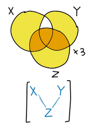
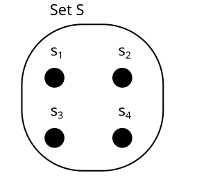
I am confused about the last correspondence between Venn Diagram and BN equivalence class (this one: ). The graph X-Z-Y implies that X⊥Y|Z. Could you explain how the Venn diagram encodes this independence/orthogonality?
I would love to see something like the Charity Entrepreneurship incubation program for AI safety.
Thanks for writing this! I agree.
I used to think that starting new AI safety orgs is not useful because scaling up existing orgs is better:
And yet, existing org do not just hire more people. After talking to a few people from AIS orgs, I think the main reason is that scaling is a lot harder than I would intuitively think.
We also see the effects of coordination costs/"scaling being hard" in industry, where there is a pressure towards people working longer hours. (It's not common that companies encourage employees to work part-time and just hire more people.)
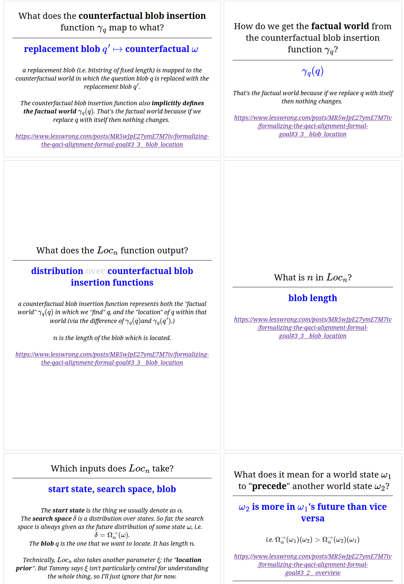
I made a deck of Anki cards for this post - I think it is probably quite helpful for anyone who wants to deeply understand QACI. (Someone even told me they found the Anki cards easier to understand than the post itself)
You can have a look at the cards here, and if you want to study them, you can download the deck here.
Here are a few example cards:
What is the procedure by which we identify the particular set factorization that models our distribution?
There is not just one factored set which models the distribution, but infinitely many. The depicted model is just a prototypical example.
The procedure for finding causal relationships (e.g. in our case) is not trivial. In that part of his post, Scott sounds like it's
1. have the suspicion that
2. prove it using the histories
I think there is probably a formalized procedure to find causal relationships using factored sets, but I'm not sure if it's written up somewhere.
For causal graphs, I don't know if there is a formalized procedure to find causal relationships which take into account all possible ways to define variables on the sample space. My general impression is that causal graphs become pretty unwieldy once we introduce deterministic nodes. And then many rules we usually use with causal graphs don't hold anymore, and working with graphs then becomes really unintuitive.
So my intuition is that yes, finding causal relationships while taking into account all possible ways to define variables is easier with factored sets than with causal graphs. (And I'm not even sure if it's even possible in general with causal graphs.) But my intuition on this isn't based on knowing a formal procedure for finding causal relationships, it just comes from my impression when playing around with the two different representations.
Possibly! Extending factored sets to continuous variables is an active area of research.
Scott Garrabrant has found 3 different ways to extend the orthogonality and time definitions to infinite sets, and it is not clear which one captures most of what we want to talk about.
About his central result, Scott writes:
I suspect that the fundamental theorem can be extended to finite-dimensional factored sets (i.e., factored sets where |B| is finite), but it can not be extended to arbitrary-dimension factored sets
If his suspicion is right, that means we can use factored sets to model continuous variables, but not model a continuous set of variables (e.g. we could model the position of a point in space as a continuous random variable, but couldn't model a curve consisting of uncountably many points)
The Countably Factored Spaces post also seems very relevant. (I have only skimmed it)
Suggestion for a different summary of my post:
Finite Factored Sets are re-framing of causality: They take us away from causal graphs and use a structure based on set partitions instead. Finite Factored Sets in Pictures summarizes and explains how that works. The language of finite factored sets seems useful to talk about and re-frame fundamental alignment concepts like embedded agents and decision theory.
I'm not completely happy with
Finite factored sets are a new way of representing causality that seems to be more capable than Pearlian causality, the state-of-the-art in causality analysis. This might be useful to create future AI systems where the causal dynamics within the model are more interpretable.
because
Consider the graph Y<-X->Z. If I set Y:=X and Z:=X
I would say then the graph is reduced to the graph with just one node, namely X. And faithfulness is not violated because we wouldn't expect X⊥X|X to hold.
In contrast, the graph X-> Y <- Z does not reduce straightforwardly even though Y is deterministic given X and Z, because there are no two variables which are information equivalent.
I'm not completely sure though if it reduces in a different way, because Y and {X, Z} are information equivalent (just like X and {Y,Z}, as well as Z and {X,Y}). And I agree that the conditions for theorem 3.2. aren't fulfilled in this case. Intuitively I'd still say X-> Y <- Z doesn't reduce, but I'd probably need to go through this paper more closely in order to be sure.
Would it be possible to formalize "set of probability distributions in which Y causes X is a null set, i.e. it has measure zero."?
We are looking at the space of conditional probability table (CPT) parametrizations in which the indepencies of our given joint probability distribution (JPD) hold.
If Y causes X, the independencies of our JPD only hold for a specific combination of conditional probabilities. Namely those in which P(X,Z) = P(X)P(Z). The set of CPT parametrizations with P(X,Z) = P(X)P(Z) has measure zero (it is lower-dimensional than the space of all CPT parametrizations).
In contrast, any CPT parametrization of graph 1 would fulfill the independencies of our given JPD. So the set of CPT parametrizations in which our independencies hold has a non-zero measure.
There are results that show that under some assumptions, faithfulness is only violated with probability 0. But those assumptions do not seem to hold in this example.
Could you say what these assumptions are that don't hold here?
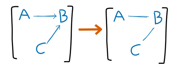
Are you sure the "arrow forgetting" operation is correct?
You say there should be an arrow when
wherein [Ni]=[A→B←C] here, and [Nj]=[A−B−C]. If we take a distribution in which A⊥/C|B , then Nj is actually a worse approximation, because A⊥C|B must hold in any distribution which can be expressed by a graph in [Nj] right?
Also, I really appreciate the diagrams and visualizations throughout the post!