(Thanks to Adam Scherlis, Kshitij Sachan, Buck Shlegeris, Chris Olah, and Nicholas Schiefer for conversations that informed this post. Thanks to Aryan Bhatt for catching an error in the loss minimization.)

Anthropic recently published a paper on toy models of superposition [Elhage+22]. One of the most striking results is that, when features are sparse, feature embeddings can become divided into disjoint subspaces with just a few vectors per subspace. This type of decomposition is known as a tegum product.

This post aims to give some intuition for why tegum products are a natural feature of the minima of certain loss functions.

Setup

Task

Suppose we’ve got $d$ embedding dimensions and $n>d$ features. We want to embed features into dimensions in a way that minimizes overlap between their embedding vectors. In the simplest case this could be because we’re building an autoencoder and want to compress the features into a low-dimensional space.

One approach is to encode all of the features in all of the dimensions. With this approach there is some interference between every pair of features (i.e. no pair is embedded in a fully orthogonal way), but we have a lot of degrees of freedom that we can use to minimize this interference.

Another approach is to split the $d$ dimensions into $k$ orthogonal subspaces of $d/k$ dimensions. This has the advantage of making most pairs of vectors exactly orthogonal, but at the cost that some vectors are packed more closely together. In the limit where $k=1$ this reduces to the first approach.

Our aim is to figure out the $k$ that minimizes the loss on this task.

Loss

Suppose our loss has the following properties:

1. $L={\sum }_{i\ne j}\ell \left(\cos {\theta }_{ij}\right)$. That is, the loss decomposes into a sum of terms involving the cosine similarities of feature vectors, and all features are equally important.
2. $\ell \left(0\right)=0$. The loss vanishes for orthogonal vectors.
3. $d\ell /d\cos \theta >0$. The loss is greater the more the vectors overlap.

Using these properties, we find that the loss is roughly

where $ϵ$ is the typical cosine similarity between vectors in a subspace.

Loss-Minimizing Subspaces

Edit: The formula for $ϵ$ below is a simplification in the limit of small $ϵ$. This simplification turns out to matter, and affects the subsequent loss minimization. I've struck through the affected sections below, explained the correct optimization in this comment below and reproduced the relevant results below the original here. None of the subsequent interpretation is affected.

The Johnson-Lindenstrauss lemma says that we can pack $m$ nearly-orthogonal vectors into $D$ dimensions, with mutual angles satisfying

where

and ${ϵ}_0$ is a constant. Setting $m=n/k$ and $D=d/k$ gives

Assuming we pick our vectors optimally to saturate the Johnson-Lindenstrauss bound, we can substitute this for $ϵ$ in the loss and differentiate with respect to $k$ to find

There are three possible cases: either the minimum occurs at $k=d$ (the greatest value it can take), or at $k=1$ (the smallest value it can take) or at some point in between where $dL/dk$ vanishes.

The derivative vanishes if

 which gives

where

When $\alpha \ge 2$ there is no place where the derivative vanishes, and the optimum is $k=1$. Otherwise there is an optimum at

so long as this is less than $d$. If it reaches $d$, the optimum sticks to $k=d$.

The Johnson-Lindenstrauss lemma says that we can pack $m$ nearly-orthogonal vectors into $D$ dimensions, with mutual angles satisfying

where ${ϵ}^2/2-{ϵ}^3/3\ge 4\log m/D$ (per Scikit and references therein). The cubic term matters because it makes the interference grow faster than the quadratic alone would imply (especially in the vicinity of $ϵ\approx 1$).

With this correction it's not feasible to do the optimization analytically, but we can still do things numerically. Setting $m=n/k$,  $D=d/k$, $n={10}^5$, and $d={10}^4$ gives:

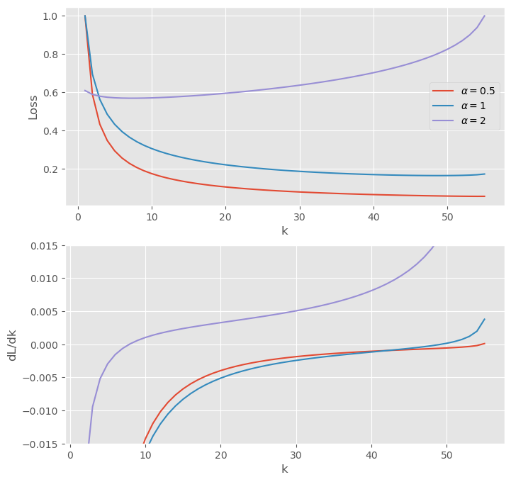
The top panel shows the normalized loss for a few different $\alpha \le 2$, and the lower shows the loss derivative with respect to $k$. Note that the range of $k$ is set by the real roots of ${ϵ}^2/2-{ϵ}^3/3\ge 4\log m/D$: for larger $k$ there are no real roots, which corresponds to the interference $ϵ$ crossing unity. In practice this bound applies well before $k\to d$. Intuitively, if there are more vectors than dimensions then the interference becomes order-unity (so there is no information left!) well before the subspace dimension falls to unity.

Anyway, all of these curves have global minima in the interior of the domain (if just barely for $\alpha =0.5$), and the minima move to the left as $\alpha$ rises. That is, for $\alpha \le 2$ we care increasingly about higher moments as we increase $\alpha$ and so we want fewer subspaces.

What happens for $\alpha >2$?

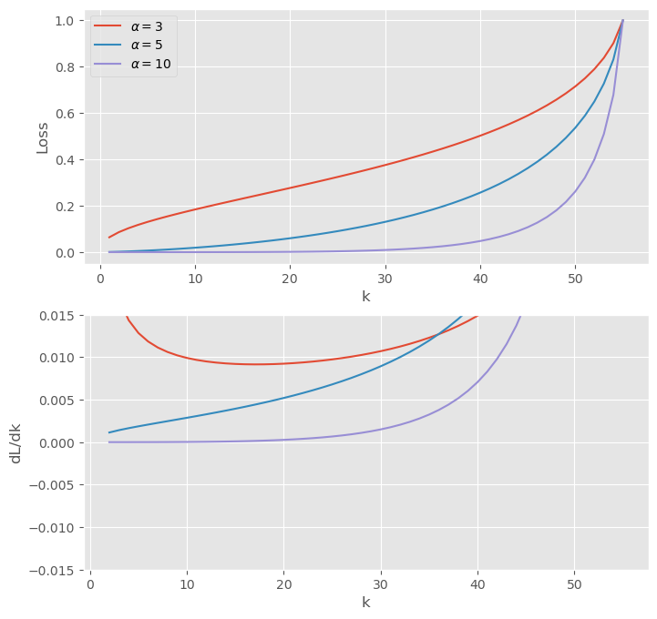
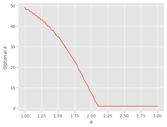
The global minima disappear! Now the optimum is always $k=1$. In fact though the transition is no longer at $\alpha =2$ but a little higher:

Interpretation

We can think of $\alpha$ as the sensitivity of the loss to interference. Specifically, which moment of the interference distribution do we care about?

When $\alpha$ is large, we care more about decreasing higher moments, and in the limit of infinite $\alpha$ what matters is just the maximum interference between vectors. Hence when $\alpha$ is large we want to have fewer subspaces, each with more vectors but smaller cosine similarities.

By contrast, when $\alpha$ is small, we care more about decreasing smaller moments, and in the limit as $\alpha \to 0$ what matters is the fraction of vectors that interfere at all. Hence when $\alpha$ is small we want to have more subspaces, each with fewer vectors but larger cosine similarities.

So tegum products are preferred when we can tolerate larger “peak” interference and want fewer instances of interference, whereas a single large subspace is preferred when we can tolerate lots of instances of interference and want to minimize the worst cases.

Relation to Anthropic’s Results

In Anthropic’s Toy Model 2, the dimension of the subspaces increases the sparser the features get, meaning that $k$ falls. We can make sense of this by expanding the loss as they do in powers of the sparsity $S$:

where $L_i$ is the loss associated with $i$-sparse vectors. In the sparse limit $S\to 1$ so

The term $L_0$ is a penalty on positive biases and the term $L_1$ is the loss on 1-sparse vectors. In this limit, the biases are negative (to minimize $L_0$), and this has the effect of wiping out the contribution of small interference terms in $L_1$. So the model is pushed to decrease the worst case interference (which might overcome the bias) rather than minimize the average, corresponding to our large-$\alpha$ limit.

On the other hand, in the dense limit $S\to 0$ so

The term $L_n$ is the loss on dense vectors, which means there is interference between all pairs of vectors. This makes minimizing the average interference more important than minimizing the really bad cases (i.e. higher moments), so the model prefers lots of small subspaces, corresponding to our small-$\alpha$ limit.

Just as the relevant limit varies with sparsity for a given toy model, we can also get different phenomenology for different models. This makes sense given that different setups can have different loss functions.

Summary

There are many ways for models to embed features. A surprising observation from Elhage+22 is that sometimes the optimal choice is one which divides the embedding space into many orthogonal subspaces (i.e. a tegum product). We can understand this roughly as coming from a tradeoff between minimizing higher moments of the feature interference (e.g. worst-case) and minimizing lower moments (e.g. average-case interference).

Smaller subspaces minimize the lower moments by making most pairs of vectors exactly orthogonal. The cost of this is that there is less freedom to choose vector pairs in each subspace, so there is worse interference between the pairs that do interfere.

Larger subspaces have the reverse tradeoff: they experience interference between more pairs of vectors, but it tends to be milder because larger-dimensional spaces support packing more nearly-orthogonal vectors, even at a fixed ratio of vectors-to-dimension.