Current best guess: Nearly all the time.
"Correlation ⇏ Causation" is trite by now. And we also know that the contrapositive is false too: "¬Correlation ⇏ ¬Causation".
Spencer Greenberg summarizes:
All of this being said, while causation does not NECESSARILY imply correlation, causation USUALLY DOES imply correlation. Some software that attempts to discover causation in observational data even goes so far as to make this assumption of causation implying correlation.
I, however, have an inner computer scientist.
And he demands answers.
He will not rest until he knows how often ¬Correlation ⇒ ¬Causation, and how often it doesn't.
This can be tested by creating a Monte-Carlo simulation over random linear structural equation models with variables, computing the correlations between the different variables for random inputs, and checking whether the correlations being zero implies that there is no causation.
So we start by generating a random linear SEM with variables (code in Julia). The parameters are normally distributed with mean 0 and variance 1.
function generate_random_linear_sem(n::Int)
    g = DiGraph(n)
    for i in 1:n
        for j in (i+1):n
            if rand() < 0.5
                add_edge!(g, i, j)
            end
        end
    end
    coefficients = Dict()
    for edge in edges(g)
        coefficients[edge] = randn()
    end
    return g, coefficients
end
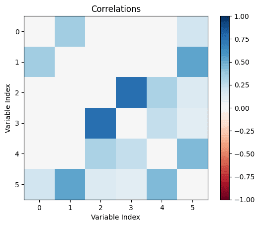
We can then run a bunch of inputs through that model, and compute their correlations:
function correlation_in_sem(sem::DiGraph, coefficients::Dict, inner_samples::Int)
    n = size(vertices(sem), 1)
    input_nodes = [node for node in vertices(sem) if indegree(sem, node) == 0]
    results = Matrix{Float64}(undef, inner_samples, n) # Preallocate results matrix
    for i in 1:inner_samples
        input_values = Dict([node => randn() for node in input_nodes])
        sem_values=calculate_sem_values(sem, coefficients, input_values)
        sem_value_row = reshape(collect(values(sort(sem_values))), 1, :)
        results[i, :] = sem_value_row
    end
    correlations=cor(results)
    for i in 1:size(correlations, 1)
        correlations[i, i] = 0
    end
    return abs.(correlations)
end
We can then check how many correlations are "incorrectly small".
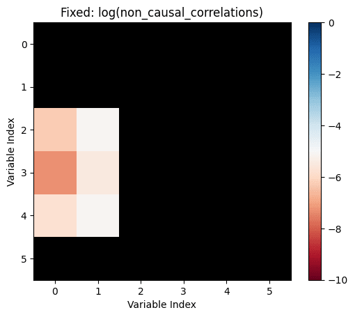
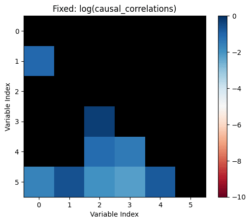
Let's take all the correlations between variables which don't have any causal relationship. The largest of those is the "largest uncaused correlation". Correlations between two variables which cause each other but are smaller than the largest uncaused correlation are "too small": There is a causation but it's not detected.
We return the amount of those:
function misclassifications(sem::DiGraph, coefficients::Dict, inner_samples::Int)
correlations=correlation_in_sem(sem, coefficients, inner_samples)
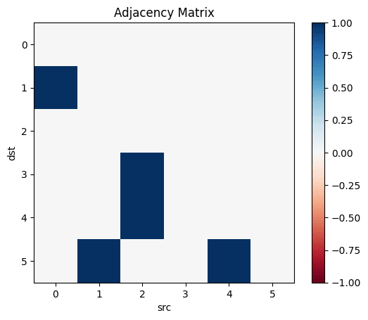
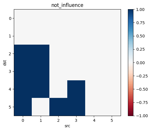
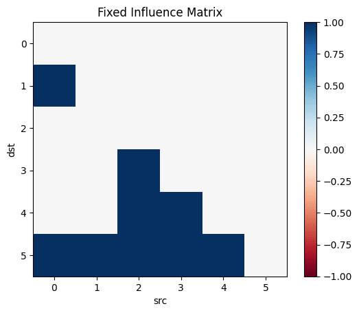
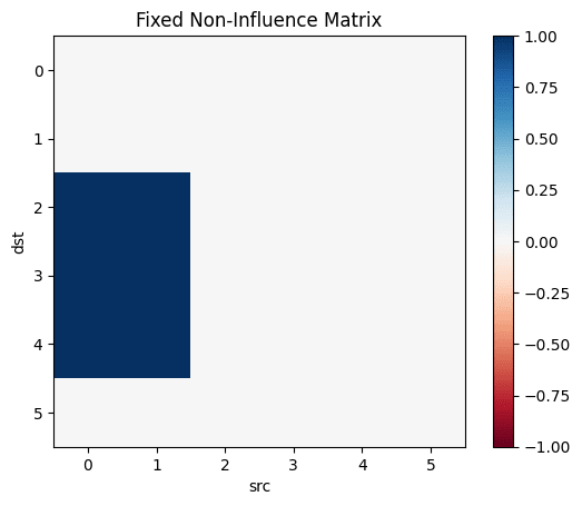
influence=Matrix(Bool.(transpose(adjacency_matrix(transitiveclosure(sem)))))
not_influence=tril(.!(influence), -1)
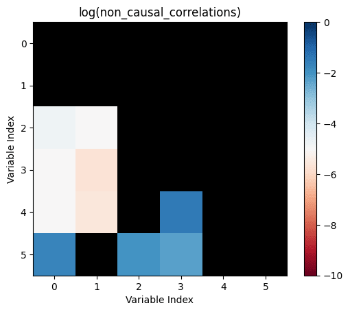
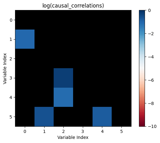
non_causal_correlations=not_influence.*correlations
causal_correlations=influence.*correlations
return sum((causal_correlations .!= 0) .& (causal_correlations .< maximum(non_causal_correlations)))
end
And, in the outermost loop, we compute the number of misclassifications for a number of linear SEMs:
    function misclassified_absence_mc(n::Int, outer_samples::Int, inner_samples::Int)
            return [misclassifications(generate_random_linear_sem(n)..., inner_samples) for i in 2:outer_samples]
    end
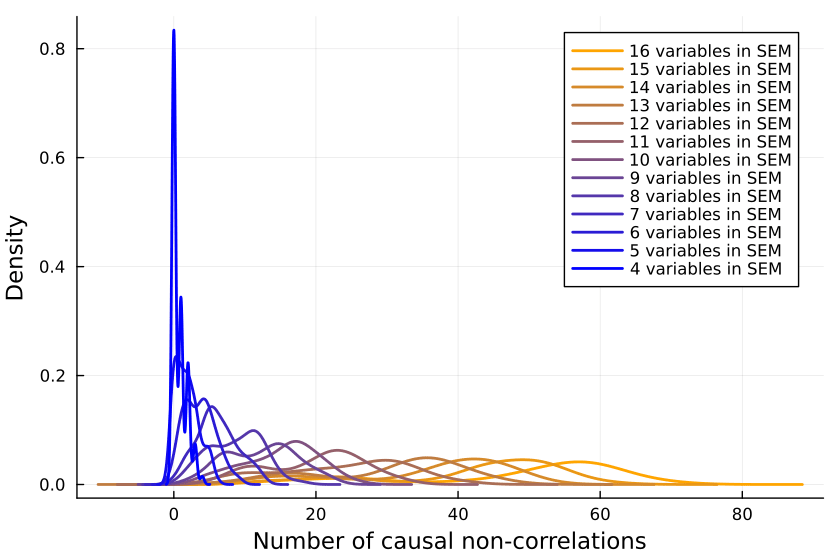
So we collect a bunch of samples. SEMs with one, two and three variables are ignored because when running the code, they never give me any causal non-correlations. (I'd be interested in seeing examples to the contrary.)
results = Dict{Int, Array{Int, 1}}()
sem_samples=200
inputs_samples=20000
for i in 4:16
    results[i]=misclassified_absence_mc(i, sem_samples, inputs_samples)
end
We can now first calculate the mean number of mistaken correlations and the proportion of misclassified correlations, using the formula for the triangular number:
    result_means=[mean(values) for (key, values) in sort(results)]
    result_props=[mean(values)/((key^2+key)/2) for (key, values) in sort(results)]
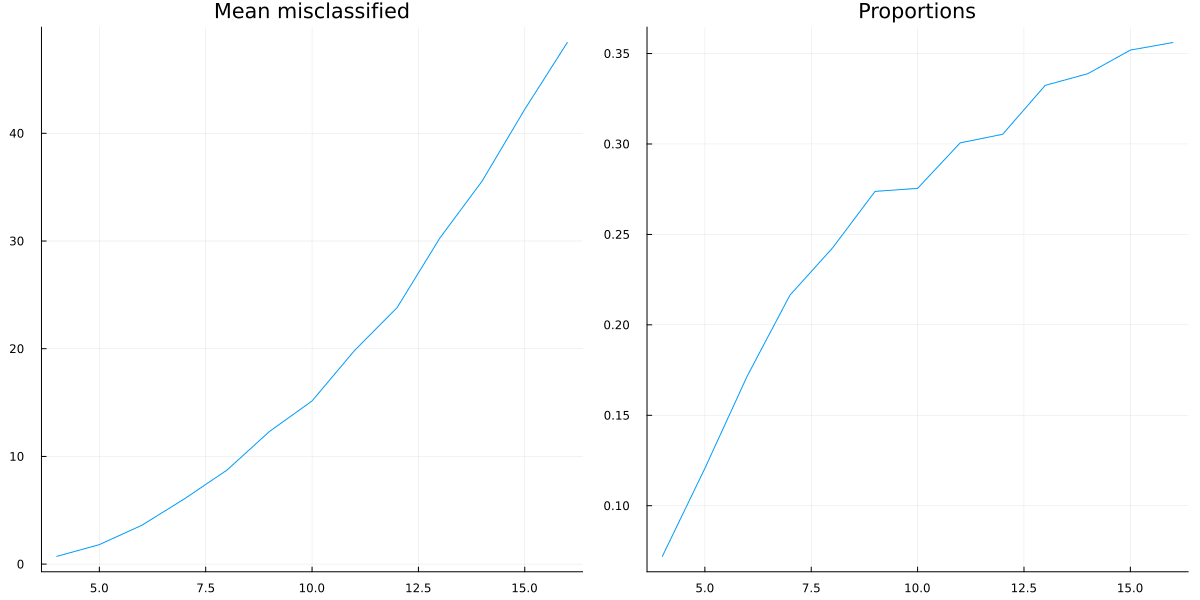
So it looks like a growing proportion of causal relationships are not correlational, and I think the number will asymptote to include almost all causal relations.
It could also be that the proportion asymptotes to another percentage, but I don't think so.
Is the Sample Size Too Small?
Is the issue with the number of inner samples, are we simply not checking enough? But 10k samples ought to be enough for anybody—if that's not sufficient, I don't know what is.
But let's better go and write some code to check:
more_samples=Dict{Int, Array{Int, 1}}()
samples_test_size=12
sem_samples=100
inputs_samples=2 .^(6:17)
for inputs_sample in inputs_samples
    println(inputs_sample)
    more_samples[inputs_sample]=misclassified_absence_mc(samples_test_size, sem_samples, inputs_sample)
end
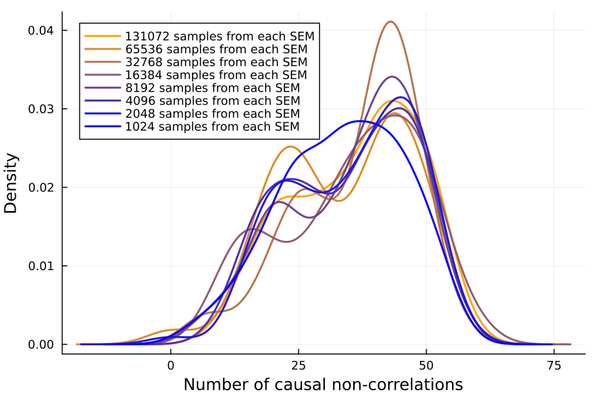
Plotting the number of causal non-correlations reveals that 10k samples ought to be enough, at least for small numbers of variables:
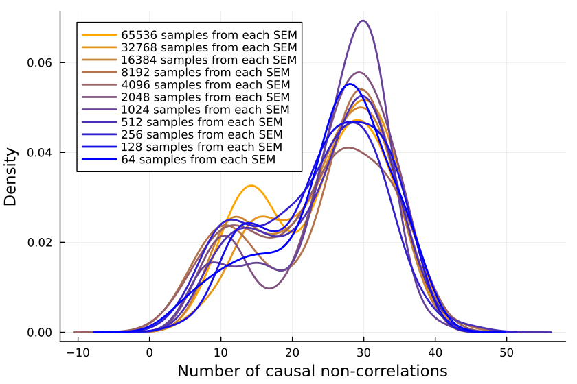
The densities fluctuate, sure, but not so much that I'll throw out the baby with the bathwater. If I was a better person, I'd make a statistical test here, but alas, I am not.

I agree with this. And yet.
The issue with that is that your "largest uncaused correlation" can be arbitrarily large -- if you've got some common factor C that explains 99% of the variance in downstream things A and B, but A does not affect B and B does not affect A, your largest uncaused correlation is going to be > 0.9 and as such you'll think that any correlations less than 0.9 are fake / undetected.
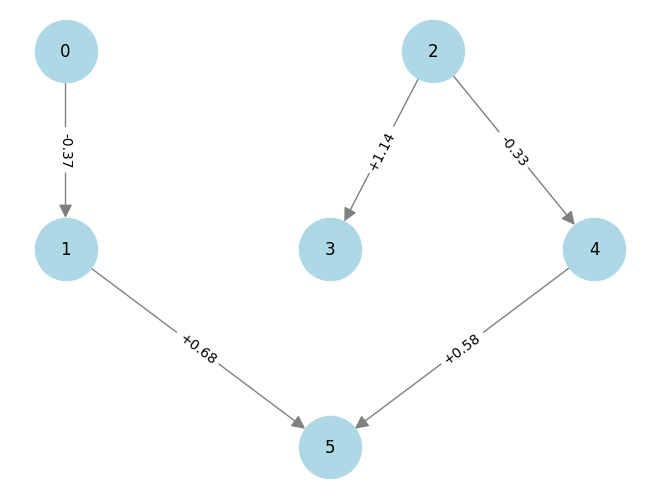
Let's make the above diagram concrete:
Let's consider the following causal influence graph
Changing the total value of vehicle registration fees collected in California will not affect the fraction of households with an electric car in Seattle, nor will changing the fraction of households with an electric car in Seattle affect the total value of vehicle registration fees collected in California. And yet we expect a robust correlation between those two.
Whether or not we can tell that past 24 hour rainfall causes changes in the spot price of electricity should not depend on the relationship between vehicle registration fees in California and electric vehicle ownership in Seattle.