There’s a common hypothesis that stochastic gradient descent has some kind of built-in bias toward simpler models, or models which generalize better. (It’s essentially the opposite of the NTK/GP/Mingard et al model.) There is also a rough intuitive argument to expect such a thing a priori: sub-structures which are only useful sometimes will be lost on the occasions when they’re not useful, whereas sub-structures which are consistently useful will be retained. Conceptually, it’s similar to the modularly varying goals model in biological evolution.
Mathematically, it’s not too hard to show that SGD does indeed have a bias, and we can even write it down explicitly given some not-too-unreasonable approximations. This post will walk through that derivation, and give some intuition for where the bias comes from.
First Idea: SGD Is Approximately Brownian
“Brownian” here refers to Brownian motion, i.e. a random walk. In other words, the path taken by SGD looks qualitatively sort of like this:
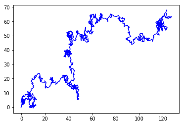
The key idea is that each sample used to estimate the gradient is approximately independent (in the probability sense of the word), and the estimate is an average over samples, so the net effect of several steps is approximately normally distributed. That’s the defining feature of Brownian motion. (Alternatively, we can assume that steps are approximately independent and additive, which gets us to the same place with a little more generality but also a little more work.)
Let’s put some math on that.
We use SGD to choose to minimize . Each step, we take independent samples of , use them to estimate the gradient, then take a step:
… where scales the step size. This step is an approximately-normal random variable, constructed from the IID random variables . It has mean , and variance .
To formally represent this as a Brownian motion, we declare that the amount-of-time which passes during each SGD step is , which we assume to be small (i.e. we’ll approximate things to first order in dt). Then SGD’s path can be represented as
… where is a standard Brownian motion, the analogue of a standard normal variable, and the square root is a matrix square root. (If you haven’t worked with Brownian motion before, ignore that formula and keep reading.)
Second Idea: Drift From High-Noise To Low-Noise Regions
Sometimes, the “noise” in a Brownian system is location-dependent. As an example, let’s consider the original use-case: a grain of pollen floats in water. It’s small enough to get randomly kicked around by water molecules, so its path is Brownian (and can be seen under an ordinary microscope). If the water has a temperature gradient, then the “noise” in the pollen-grain’s path will vary with its location.
When the grain of pollen is in a higher-noise region, it will be kicked around more, and move around faster, until eventually it moves into a lower-noise region. In the lower-noise region, it will be kicked around less, and move around slower, so it takes longer to leave the region. So, the pollen grain will tend to spend more time in lower-noise regions. With a noise gradient, this tendency to spend more time in lower-noise regions becomes a tendency to drift down the noise gradient.

Mathematically, if is our pollen location, we can write its motion as
… for a location-dependent “drift” , “diffusion matrix” (larger in higher temperature regions), and is the standard Brownian motion again. Intuitively, the “drift” pushes along the direction , and the “diffusion” controls how fast spreads out along each direction - or at least that’s how we think about it for constant drift and diffusion. The probability distribution of evolves over time according to:
(This is the Fokker-Planck equation.)
Key thing to notice: we can re-write this as
… so acts like a drift term, just like . This noise-induced drift is nonzero only when there's a noise gradient.
A very simple example of the math: suppose (i.e. it’s an identity matrix scaled by ). Then . So, the diffusion-gradient-induced drift is constant and along the direction.
Putting It Together
So:
- SGD’s path is approximately-Brownian, with location-dependent noise
- Brownian motion with location-dependent noise tends to drift down the noise gradient
In SGD, our “intended” drift is - i.e. drift down the gradient of the objective. But the location-dependent noise contributes a “bias” - a second drift term, resulting from drift down the noise-gradient. Combining the equations from the previous two sections, the noise-gradient-drift is
I don’t have much theory or evidence right now for what kinds of things that bias pushes towards (other than “regions of low gradient noise”), but having an explicit formula should help investigate that sort of question. Personally, I suspect that it pushes toward models with a modular structure reflecting the modularity structure of the environment, which is the main reason I'm interested in it.
I'm still wrapping my head around this myself, so this comment is quite useful.
Here's a different way to set up the model, where the phenomenon is more obvious.
Rather than Brownian motion in a continuous space, think about a random walk in a discrete space. For simplicity, let's assume it's a 1D random walk (aka birth-death process) with no explicit bias (i.e. when the system leaves state k, it's equally likely to transition to k+1 or k−1). The rate λk at which the system leaves state k serves a role analogous to the diffusion coefficient (with the analogy becoming precise in the continuum limit, I believe). Then the steady-state probabilities of state k and state k−1 satisfy
pkλk=pk−1λk−1
... i.e. the flux from values-k-and-above to values-below-k is equal to the flux in the opposite direction. (Side note: we need some boundary conditions in order for the steady-state probabilities to exist in this model.) So, if λk>λk−1, then pk<pk−1: the system spends more time in lower-diffusion states (locally). Similarly, if the system's state is initially uniformly-distributed, then we see an initial flux from higher-diffusion to lower-diffusion states (again, locally).
Going back to the continuous case: this suggests that your source vs destination intuition is on the right track. If we set up the discrete version of the pile-of-rocks model, air molecules won't go in to the rock pile any faster than they come out, whereas hot air molecules will move into a cold region faster than cold molecules move out.
I haven't looked at the math for the diode-resistor system, but if the voltage averages to 0, doesn't that mean that it does spend more time on the lower-noise side? Because presumably it's typically further from zero on the higher-noise side. (More generally, I don't think a diffusion gradient means that a system drifts one way on average, just that it drifts one way with greater-than-even probability? Similar to how a bettor maximizing expected value with repeated independent bets ends up losing all their money with probability 1, but the expectation goes to infinity.)
Also, one simple way to see that the "drift" interpretation of the diffusion-induced drift term in the post is correct: set the initial distribution to uniform, and see what fluxes are induced. In that case, only the two drift terms are nonzero, and they both behave like we expect drift terms to behave - i.e. probability increases/decreases where the divergence of the drift terms is positive/negative.