Elhage et al at Anthropic recently published a paper, Toy Models of Superposition (previous Alignment Forum discussion here) exploring the observation that in some cases, trained neural nets represent more features than they “have space for”--instead of choosing one feature per direction available in their embedding space, they choose more features than directions and then accept the cost of “interference”, where these features bleed over into each other. (See the SoLU paper for more on the Anthropic interpretability team’s take on this.)
We (Kshitij Sachan, Adam Scherlis, Adam Jermyn, Joe Benton, Jacob Steinhardt, and I) recently uploaded an Arxiv paper, Polysemanticity and Capacity in Neural Networks, building on that research. In this post, we’ll summarize the key idea of the paper.
We analyze this phenomenon by thinking about the model’s training as a constrained optimization process, where the model has a fixed total amount of capacity that can be allocated to different features, such that each feature can be ignored, purely represented (taking up one unit of capacity), or impurely represented (taking up some amount of capacity between zero and one units).
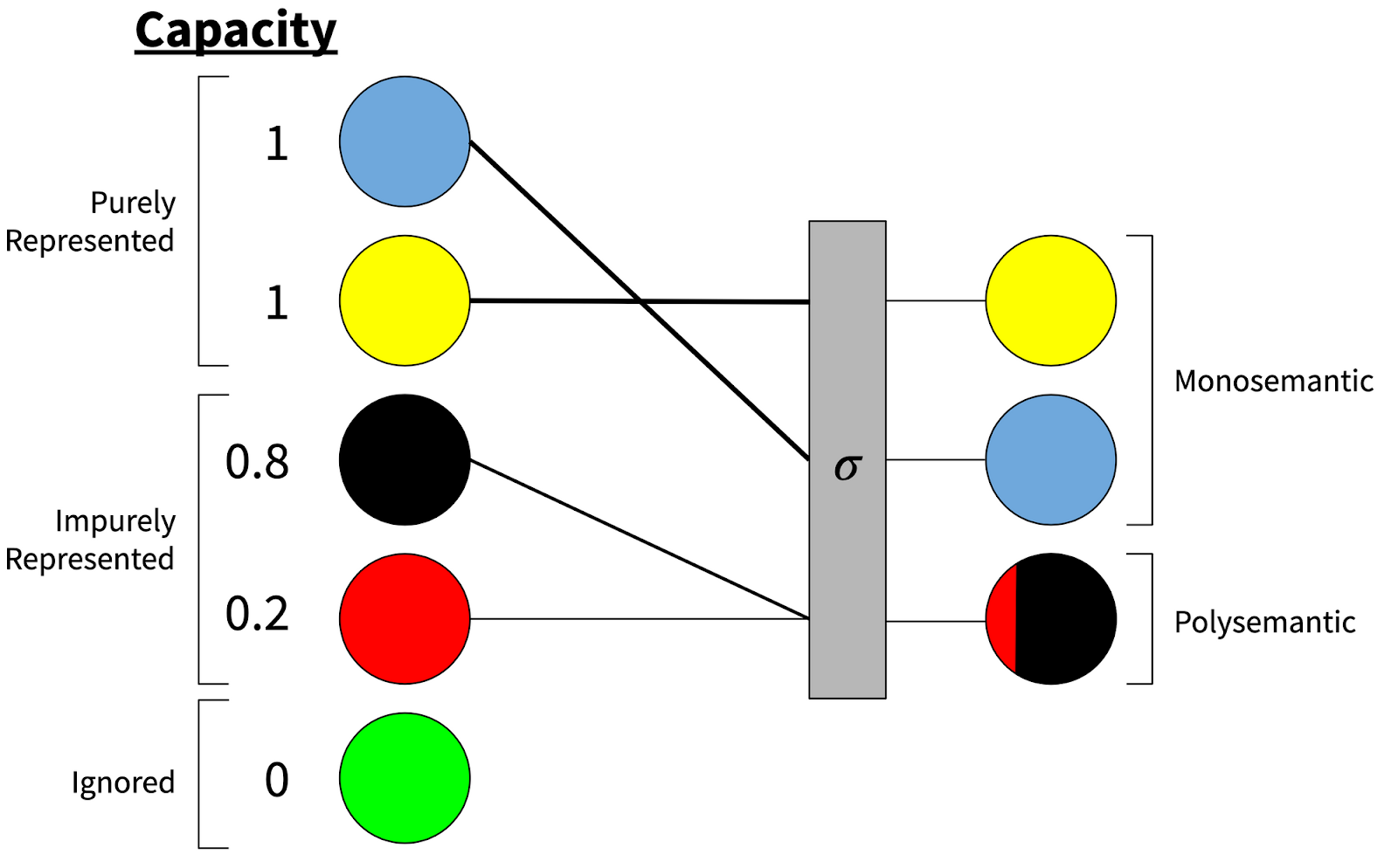
When the model purely represents a feature, that feature gets its own full dimension in embedding space, and so can be represented monosemantically; impurely represented features share space with other features, and so the dimensions they’re represented in are polysemantic.
For each feature, we can plot the marginal benefit of investing more capacity into representing that feature, as a function of how much it’s currently represented. Here we plot six cases, where one feature’s marginal benefit curve is represented in blue and the other in black.

These graphs show a variety of different possible marginal benefit curves. In A and B, the marginal returns are increasing–the more you allocate capacity to a feature, the more strongly you want to allocate more capacity to it. In C, the marginal returns are constant (and in this graph they happen to be equal for the two features, but there’s no reason why constant marginal returns imply equal returns in general). And then in D, E, and F, there are diminishing marginal returns.
Now, we can make the observation that, like in any budget allocation problem, if capacities are allocated optimally, the marginal returns for allocating capacity to any feature must be equal (if the feature isn’t already maximally or minimally represented). Otherwise, we’d want to take capacity away from features with lower dLi/dCi and give it to features with higher dLi/dCi .
In the case where we have many features with diminishing marginal returns, capacity will in general be allocated like this:
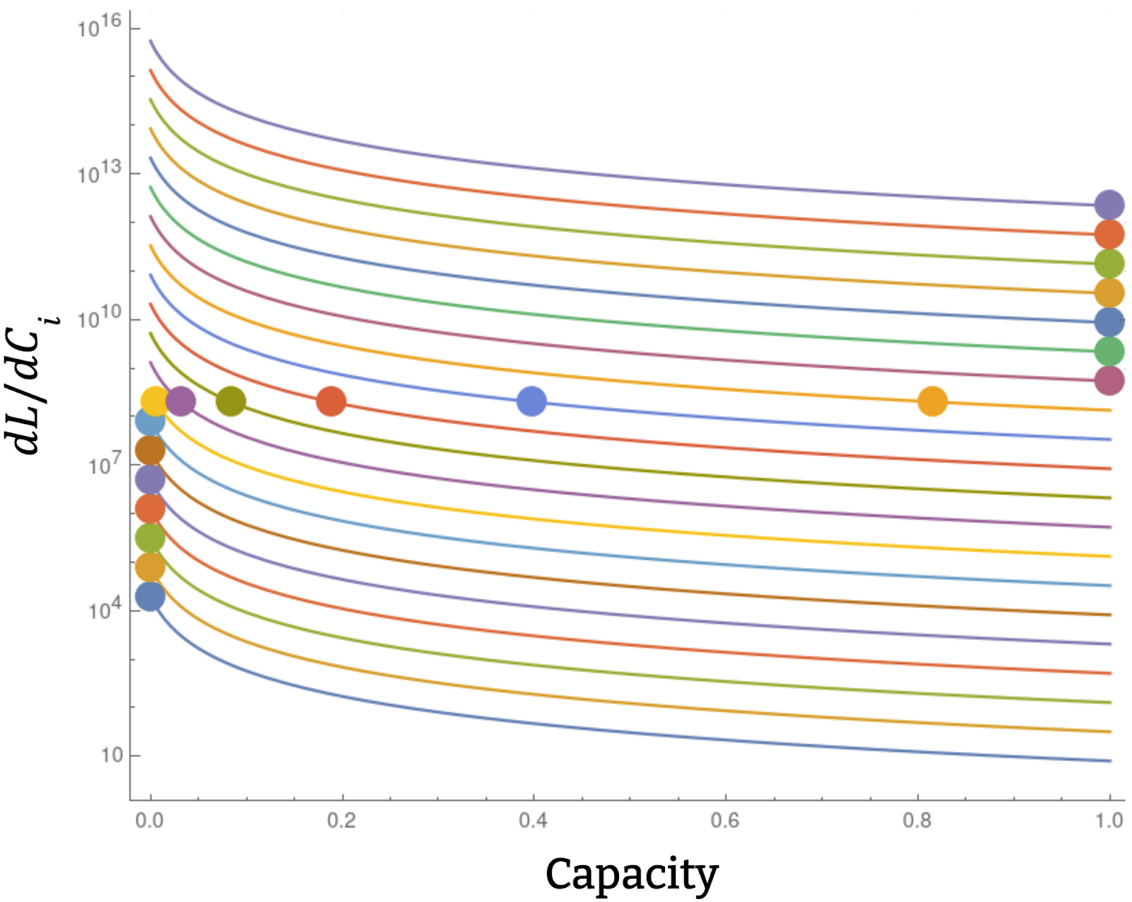
Here the circles represent the optimal capacity allocation for a particular total capacity.
This perspective suggests that polysemanticity will arise when there are diminishing marginal returns to capacity allocated to particular features (as well as in some other situations that we think are less representative of what goes on in networks).
In our paper, we do the following:
- We describe a particularly analytically tractable model which exhibits polysemanticity.
- We analyze our model using the capacity framework, derive the above graphs, and replicate them numerically.
- Elhage et al empirically observe that increasing the sparsity increases superposition. We analytically ground this observation by decomposing our toy model’s loss into two terms that directly correspond to the benefits and costs of superposition. As the input data becomes sparser, the kurtosis increases, and as the kurtosis increases the loss more heavily favors superposition.
- We explain the phase transitions observed in our model, which look similar to the phase transitions observed in Elhage et al–the sharp lines are because the capacities eventually hit 0 or 1, and at low sparsity you never see features represented impurely because the marginal returns curves don’t have diminishing returns. We can use this understanding to analytically derive the phase diagram:

- Lastly, in Elhage et al’s toy model, features were often partitioned into small distinct subspaces; we explore this as a consequence of optimal allocation of capacity: we find a block-semi-orthogonal structure, with differing block sizes in different models.
How important or useful is this? We’re not sure. For Redwood this feels like more of a side-project than a core research project. Some thoughts on the value of this work:
- We suspect that the capacity framework is getting at some important aspects of what’s going on in the training process for real neural networks, though probably the story in large models is probably substantially messier.
- We think that our results are helpful additions to the story laid out in Elhage et al.
- We think it’s nice to have some extremely simple examples where we understand polysemanticity very well. E.g. We’ve found it helpful to use our toy model as a testcase when developing interpretability techniques that should work in the presence of polysemantic neurons.

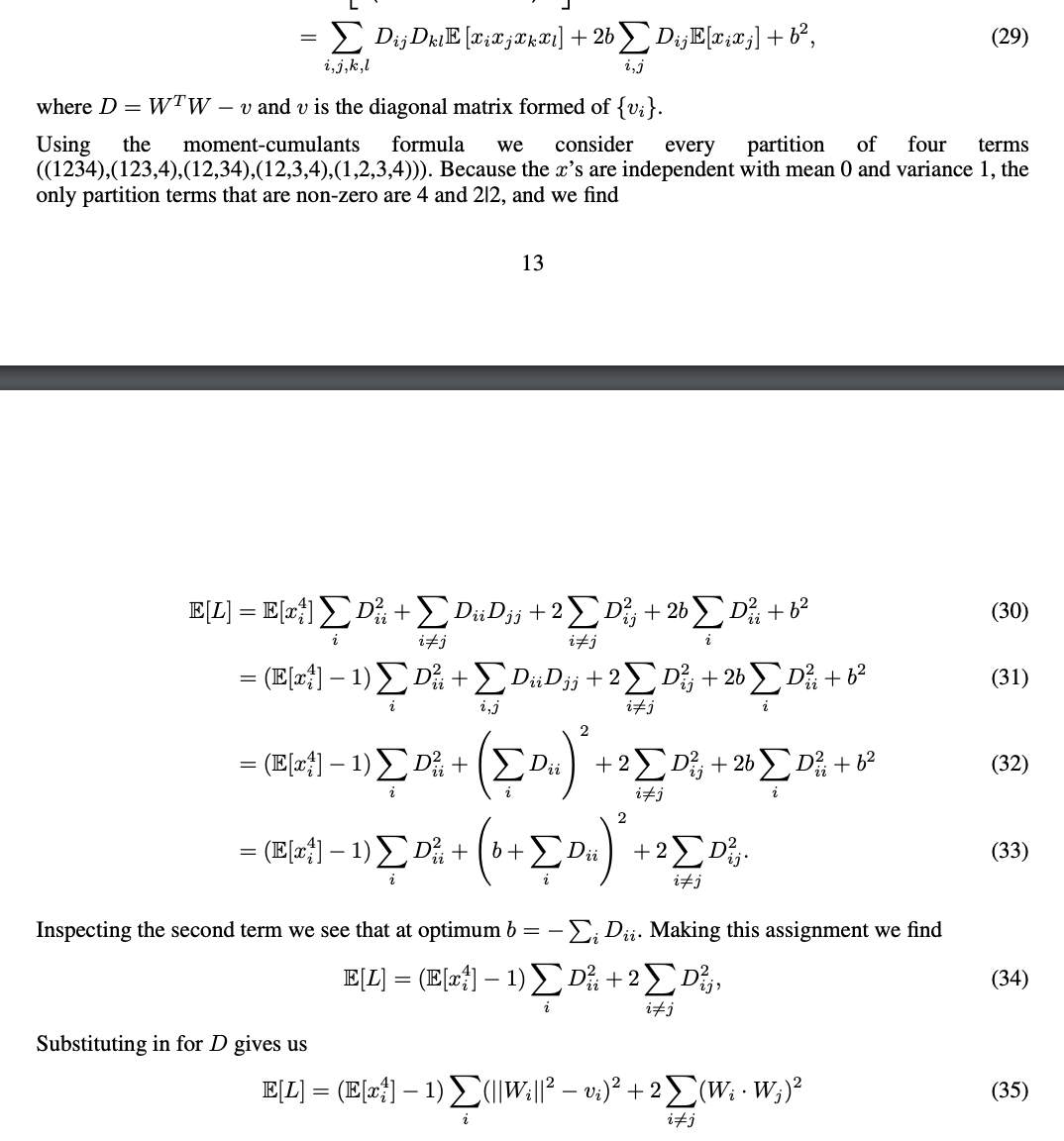

A few notes/questions about things that seem like errors in the paper (or maybe I'm confused — anyway, none of this invalidates any conclusions of the paper, but if I'm right or at least justifiably confused, then these do probably significantly hinder reading the paper; I'm partly posting this comment to possibly prevent some readers in the future from wasting a lot of time on the same issues):
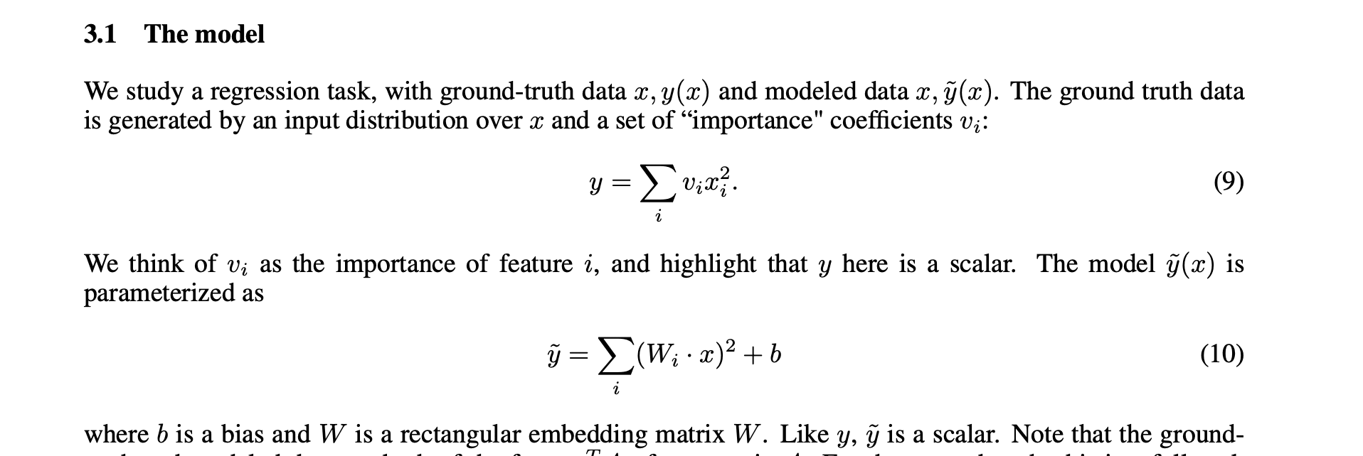
1) The formula for ~y here seems incorrect:
This is because W_i is a feature corresponding to the i'th coordinate of x (this is not evident from the screenshot, but it is evident from the rest of the paper), so surely what shows up in this formula should not be W_i, but instead the i'th row of the matrix which has columns W_i (this matrix is called W later). (If one believes that W_i is a feature, then one can see this is wrong already from the dimensions in the dot product Wi⋅x not matching.)
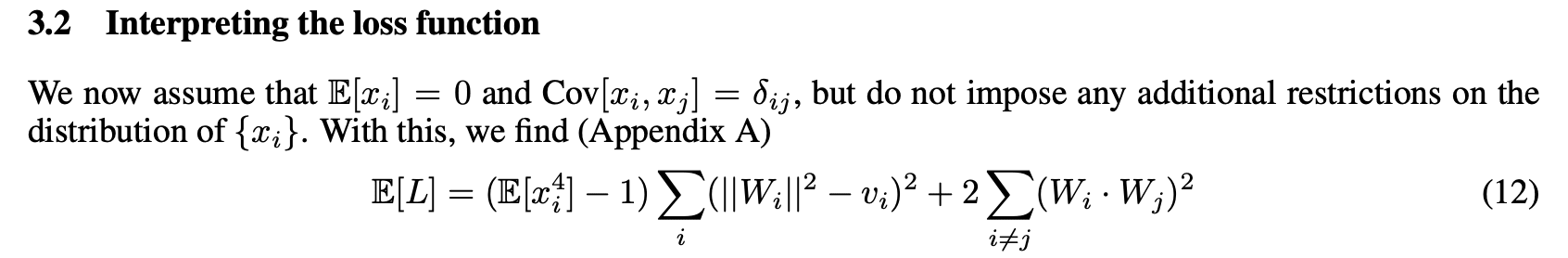
2) Even though you say in the text at the beginning of Section 3 that the input features are independent, the first sentence below made me make a pragmatic inference that you are not assuming that the coordinates are independent for this particular claim about how the loss simplifies (in part because if you were assuming independence, you could replace the covariance claim with a weaker variance claim, since the 0 covariance part is implied by independence):
However, I think you do use the fact that the input features are independent in the proof of the claim (at least you say "because the x's are independent"):
Additionally, if you are in fact just using independence in the argument here and I'm not missing something, then I think that instead of saying you are using the moment-cumulants formula here, it would be much much better to say that independence implies that any term with an unmatched index is 0. If you mean the moment-cumulants formula here https://en.wikipedia.org/wiki/Cumulant#Joint_cumulants , then (while I understand how to derive every equation of your argument in case the inputs are independent), I'm currently confused about how that's helpful at all, because one then still needs to analyze which terms of each cumulant are 0 (and how the various terms cancel for various choices of the matching pattern of indices), and this seems strictly more complicated than problem before translating to cumulants, unless I'm missing something obvious.

3) I'm pretty sure this should say x_i^2 instead of x_i x_j, and as far as I can tell the LHS has nothing to do with the RHS:
(I think it should instead say sth like that the loss term is proportional to the squared difference between the true and predictor covariance.)
I've uploaded a fixed version of this paper. Thanks so much for putting in the effort to point out these mistakes - I really appreciate that!