TLDR; This is the first post of Distilling Singular Learning Theory (DSLT), an introduction to which can be read at DSLT0. In this post I explain how singular models (like neural networks) differ from regular ones (like linear regression), give examples of singular loss landscapes, and then explain why the Real Log Canonical Threshold (aka the learning coefficient) is the correct measure of effective dimension in singular models.
When a model class is singular (like neural networks), the complexity of a parameter in parameter space needs a new interpretation. Instead of being defined by the total parameters available to the model , the complexity (or effective dimensionality) of is defined by a positive rational called the Real Log Canonical Threshold (RLCT), also known as the learning coefficient. The geometry of the loss is fundamentally defined by the singularity structure of its minima, which measures. Moreover, in regular models like linear regression the RLCT is , but in singular models it satisfies in general. At its core, then, Sumio Watanabe's Singular Learning Theory (SLT) shows the following key insight:
The RLCT is the correct measure of effective dimensionality of a model .
Watanabe shows that the RLCT has strong effects on the learning process: it is the correct generalisation of model complexity in the Bayesian Information Criterion for singular models, and therefore plays a central role in the asymptotic generalisation error, thereby inheriting the name "learning coefficient".
In this first post, after outlining the Bayesian setup of SLT, we will start by defining what a singular model is and explain what makes them fundamentally different to regular models. After examining different examples of singular loss landscapes, we will define the RLCT to be the scaling exponent of the volume integral of nearly true parameters, and conclude by summarising how this quantity correctly generalises dimensionality.
Preliminaries of SLT
The following section introduces some necessary technical terminology, so use it as a reference point, not necessarily something to cram into your head on a first read through. A more thorough setup can be found in [Car21, Chapter 2], which follows [Wat09] and [Wat18].
SLT is established in the Bayesian paradigm, where the Bayesian posterior on the parameter space is the primary object of focus, containing information on which parameters correspond to "good" models.
Our statistical learning setup consists of the following data:
- A dataset , where for each is an input and is an output (so we are in the supervised learning setting).
- We suppose the sequence in is independent and identically distributed according to a true distribution . For our purposes, we assume the true distribution of inputs to be known, but the true distribution of outputs to be unknown.
- We then choose a model class defined by parameters in a compact parameter space that contains the origin. We hope to find model parameters that will adequately approximate the truth, or in other words, learn how to accurately predict an output given an input. For example, a model class could be a fixed neural network architecture with Gaussian noise, as below.
- We can select a prior distribution of our choosing[1] that is non-zero on , so .
Using this data, the error of the model on the dataset is defined by the empirical negative log likelihood (NLL), ,
where is the model likelihood. [2] [3]
This gives rise to the Bayesian posterior of defined by [4]
where the partition function (or in Bayesian terms the evidence) is given by
The partition function measures posterior density, and thus contains a lot of macroscopic data about a system. Inspired by its role in physics, and for theoretical ease, we consider the free energy
Performing asymptotic analysis on (and therefore ) is the main task of SLT. The learning goal is to find small regions of parameter space with high posterior density, and therefore low free energy.
Though we never have access to the truth in the learning procedure, for theoretical purposes we nonetheless define the empirical entropy of the true distribution
Even though this quantity is always inaccessible in real settings, there is almost sure convergence as to a constant that doesn't depend on , [5]
To study the posterior, we define the Kullback-Leibler divergence between the truth and the model,
which is the infinite-data limit of its empirical counterpart,
The KL divergence is usually thought of as a "loss metric"[6] between the truth and and the model since
- for all , and;
- if and only if for all and all .
As such, I will colloquially refer to as the loss landscape. [7] The current state of results in SLT require to be an analytic function, but it seems likely that the results can be generalised to non-analytic settings with suitable hypotheses and constraints.
To analyse where the loss is minimised, we are then lead to defining the set of true parameters,
We say that the true distribution is realisable by the model class if is non empty, that is, there exists some such that for all . Despite being unrealistic in real world applications, this is nonetheless an important starting point to the theory, which will then generalise to the set of optimal parameters in DSLT2.
We are going to restrict our attention to a particular kind of model: neural networks with Gaussian noise. We will formally define a neural network in a following chapter of this sequence, but for now it suffices to say that it is a function with inputs and outputs defined by some parameter . Then our model density is going to be given by
From here on in, we will assume we are working with a (model, truth, prior) triple as specified in this section.
Loss in our setting
To put these technical quantities into perspective, let me make clear two key points:
- Under the regression model, the NLL is equivalent to the mean-squared error of the neural network on the dataset (up to a constant),
- In the realisable case where , the KL divergence is just the euclidean distance between the model and the truth adjusted for the prior measure on inputs,
Singular vs Regular Models
What is a singular model?
The key quantity that distinguishes regular and singular models is the Fisher information matrix , whose entries are defined by
It can be shown that when evaluated at a point on the set of true parameters , the Fisher information matrix is simply the Hessian of , so
A regular statistical model class is one which is identifiable (so implies that ), and has positive definite Fisher information matrix for all . Regular model classes, such as standard linear regression, are the backbone of classical statistics for which all pre-exisiting literature on Bayesian statistics applies. But, from the point of view of SLT, regular model classes are... boring.
If a model class is not regular, then it is strictly singular. The non-identifiability condition can be easily dealt with, but it is the degeneracy of the Fisher information matrix that fundamentally changes the nature of the posterior and its asymptotics. We will say a model defined by a fixed (not necessarily a true parameter) is strictly singular if the Fisher information at the point, , is degenerate, meaning
- , where is the number of dimensions in parameter space , or equivalently;
- .
Then the model class is strictly singular if there exists a such that is degenerate. A singular model class can be either regular or strictly singular - Watanabe's theory thus generalises regular models, regardless of the model non-identifiability or degenerate Fisher information.
It can be easily shown that, under the regression model, is degenerate if and only the set of derivatives
is linearly dependent.
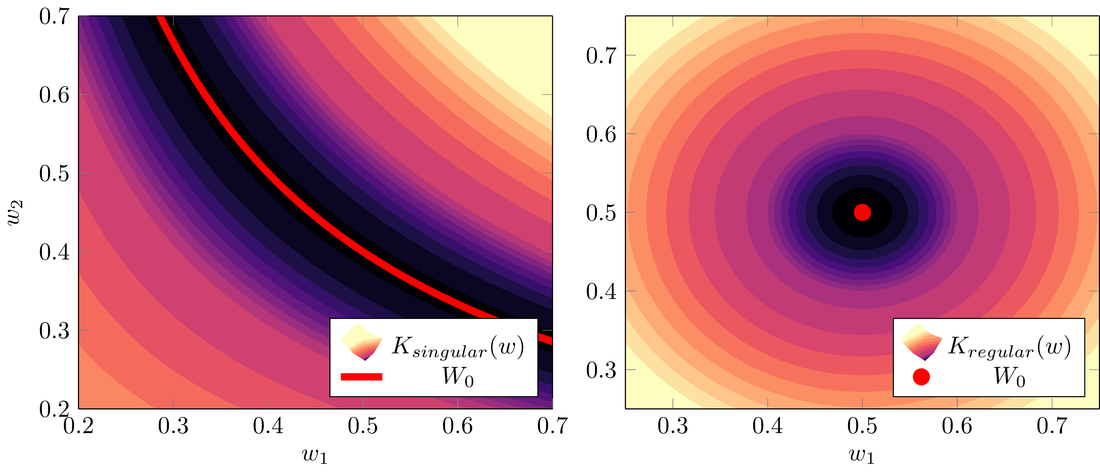
In regular models, the set of true parameters consists of one point. But in singular models, the degeneracy of the Fisher information matrix means is not restricted to being one point, or even a set of isolated points - in general, these local minima of are connected together in high-dimensional structures [8]. In strictly singular models, the true parameters are degenerate singularities [9] of , and thus cannot be approximated by a quadratic form near these points. This is the fundamental reason the classical theory of Bayesian statistics breaks down.
Watanabe states that "in singular statistical models, the knowledge or grammar to be discovered corresponds to singularities in general" [Wat09]. With this in mind, it is unsurprising that the following widely used models are all examples of singular models:
- Layered neural networks
- Gaussian, binomial, multinomial and other mixture models
- Reduced rank regression
- Boltzmann machines
- Bayes networks
- Hidden Markov models
Singular models are characterised by features like: having hierarchical structure, being made of superposition of parametric functions, containing hidden variables, etc., all in the service of obtaining hidden knowledge from random samples.
Classical Bayesian inference breaks down for singular models
There are two key properties of regular models that are critical to Bayesian inference as :
- Asymptotic normality: The posterior of regular models converges in distribution to a -dimensional normal distribution centred at the maximum likelihood estimator [Vaa07]:
- Bayesian Information Criterion (BIC): The free energy of regular models asymptotically looks like the BIC as , where and is the dimension of parameter space :
At the core of both of these results is an asymptotic expansion that strongly depends on the Fisher information matrix being non-degenerate at true parameters . It's instructive to see why this is, so let's derive the BIC to see where shows up.
Deriving the Bayesian Information Criterion only works for regular models
For the sake of this calculation, let us assume . Taking our cues from [Kon08], suppose (thus is a maximum likelihood estimator and satisfies ). We can Taylor expand the NLL as
where is the Hessian. Since we are analysing the asymptotic limit , we can relate this Hessian to the Fisher information matrix,
By definition is a minimum of , so , so we can expand the partition function as
Here's the crux: if is non-degenerate (so the model is regular), then we can perform this integral in good-faith knowing that it will always exist. In that case, the second term involving vanishes since it is the first central moment of a normal distribution, so we have
since the integrand is the integral of a -dimensional multivariate Gaussian . Notice here that this is the same distribution that arises in the asymptotic normality result, a theorem that has the same core, but requires more rigorous probability theory to prove. If is degenerate, then it is non-invertible, meaning the above formulas cannot hold.
The free energy of this ensemble is thus
and so ignoring terms less than in , we arrive at the Bayesian Information Criterion
This quantity can be understood as an accuracy-complexity tradeoff, where the complexity of the model class is defined by . We will elaborate on this more in DSLT2 but for now, you should just believe that the Fisher information is a big deal. Generalising this procedure (and therefore the BIC) for singular models, is the heart of SLT.
Examples of Singular Loss Landscapes
In essence, the Fisher information matrix describes something about the effective dimensionality or complexity of a model . When a model class is regular, the effective dimensionality of every point is simply , the number of parameters available to the model. But in the singular case, a new notion of effective dimensionality is required to adequately describe the complexity of a model. We're now going to look at two cases of singular models [10] - or more precisely, loss landscapes that correspond to singular models - to motivate this generalisation. We'll start with the easier case where one or more parameters are genuinely "free".
Sometimes singularities are just free parameters
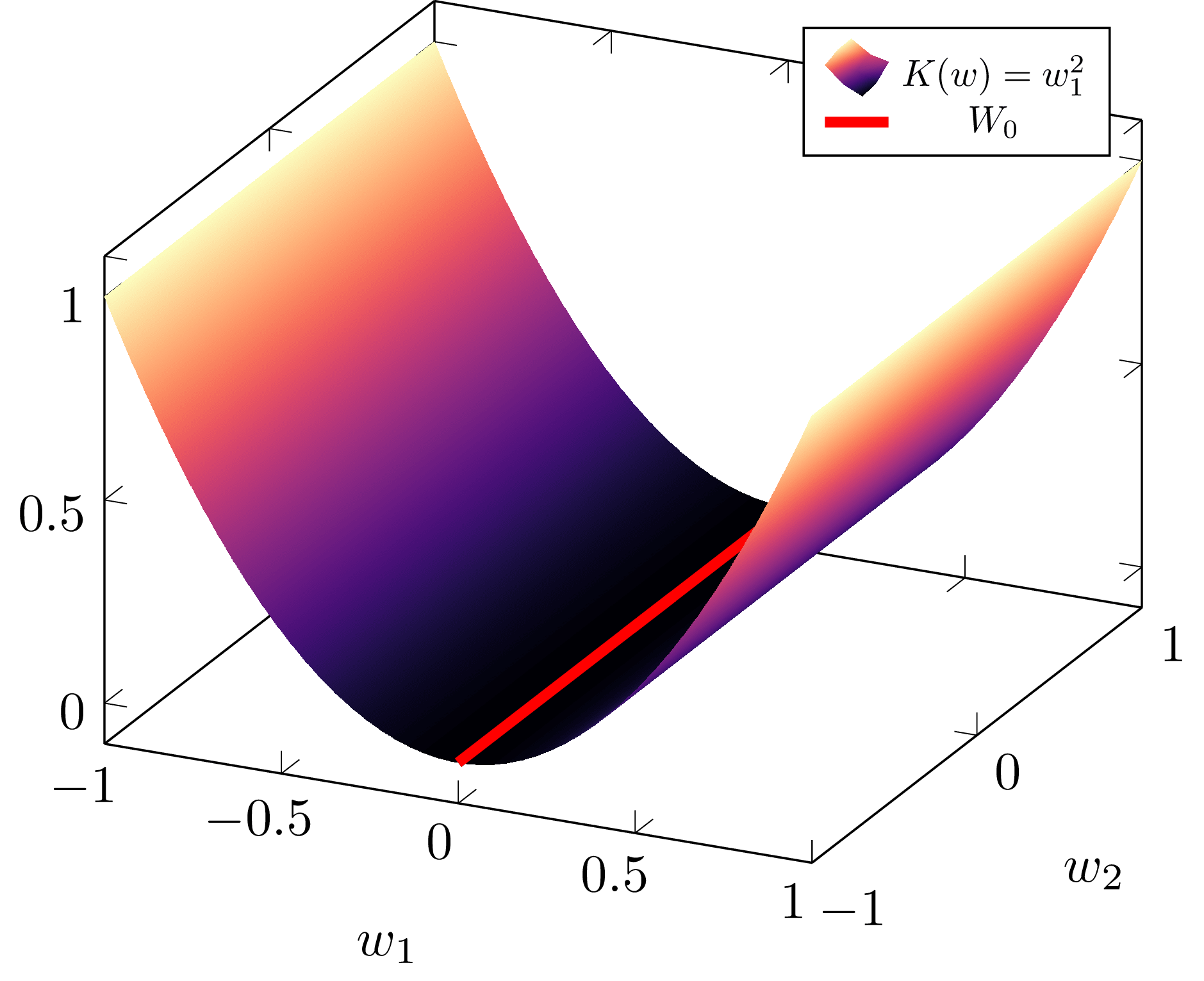
Example 1.1: Suppose we have parameters afforded to a model such that , which has a Hessian given by
Taking the critical point , we have and so , thus the model is singular. In this case, since for all , we could simply throw out the free parameter and define a regular model with parameters that has identical geometry , and therefore defines the same input-output function, .
This example is called a minimally singular case. Suppose with integers such that , and after some change of basis[11] we may write a local expansion of as the sum of squares,
where are positive coefficients. Then the Fisher information matrix has the form
where is the square zero matrix. Perhaps then we could define the "effective dimensionality" of as being , which is the number of tangent directions in parameter space in which the model changes - the number of "non-free" parameters - and just discard the "free" parameters that are normal to
Sure! We can do that, and if we did, our BIC derivation would carry out fine and we would just replace by in the final formula. So the minimally singular case is easy to handle.
But this doesn't always work.
But not all singularities are free parameters
Defining the effective dimensionality at as seems nice in theory, but turns out to give nonsensical answers pretty quickly - it is not a full enough description of the actual geometry at play.
Example 1.2: Suppose instead that . Then the Hessian is
At the critical point the Fisher information is
which is obviously degenerate.
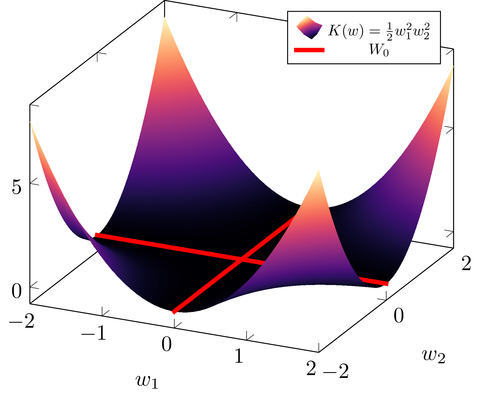
If we used our notion of effective dimensionality from before, we would say the model defined by had effective dimension of . But this would be ridiculous - clearly there are more than zero "effective dimensions" in this model, a term that would intuitively imply was identically zero, which it clearly is not. Thus, we need a different way of thinking about effective dimensionality.
The Real Log Canonical Threshold (aka the Learning Coefficient)
In this section we are going to explain the key claim of this post: that effective dimensionality in singular models is measured by a positive rational number called the Real Log Canonical Threshold, also known as the learning coefficient.
Dimensionality as a volume co-dimension
Taking inspiration from Weyl's famous Volume of Tubes paper, we can reframe dimensionality in terms of a scaling exponent of the volume of "nearly" true parameters. To explain this, we will generalise the minimally singular case above. The following discussion follows [Wei, 22].
Assume we have a partition as before with such that , where is the number of non-free parameters and is the number of free parameters. For any we can consider the set of almost true parameters centred at (which, without loss of generality, we will take to be ),
and an associated volume function

As long as the prior is non-zero on it does not affect the relevant features of the volume, so we may assume that it is a constant in the first directions and is a normal distribution in the remaining . Then since , we can write
The right integrand is some constant that doesn't depend on , and for the left we can make the substitution , hence
Recognising the integrand as the volume of the -ball, a constant that does not depend on , we see that
Then the dimension arises as the scaling exponent of , which can be extracted via the following ratio of volumes formula for some :
This scaling exponent, it turns out, is the correct way to think about dimensionality of singularities.
Watanabe shows in Theorem 7.1 of [Wat09] that in general, for any singular model defined by , the volume integral centred at has the form
where is a positive rational number called the Real Log Canonical Threshold (RLCT) associated to the "most singular point" in . This is the quantity that generalises the dimensionality of a singularity. What's more, different singularities in can have different RLCT values, and thereby different "effective dimensionalities". As suggested above, the RLCT can then be defined by this volume formula:
An example of fractional dimension
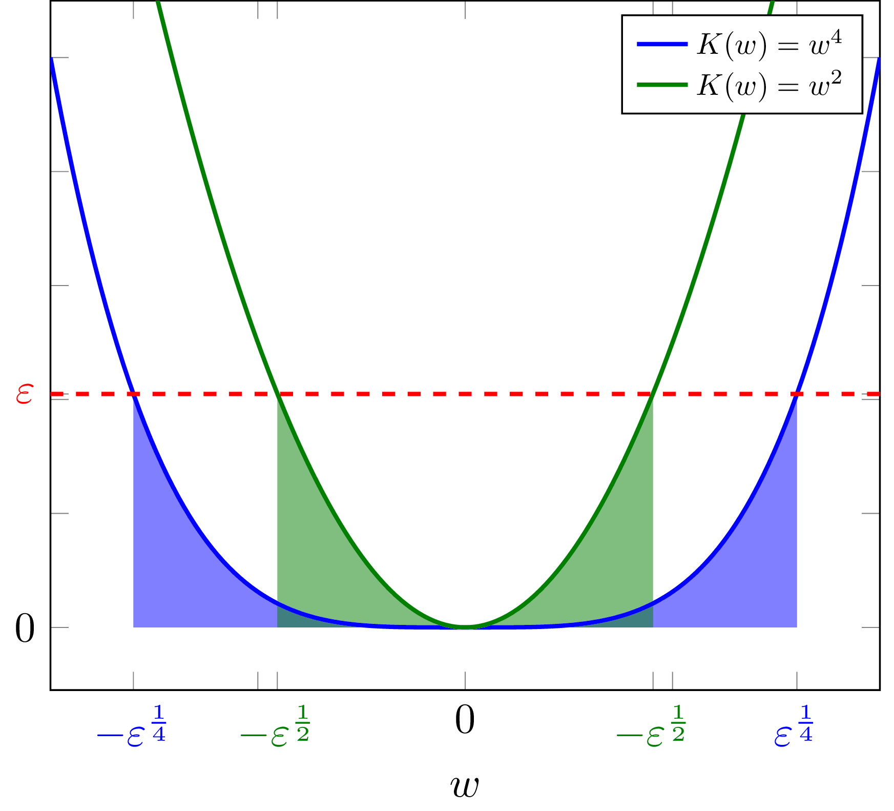
Example 1.3: To build intuition for what a "fractional dimension" is, consider a model with parameters with KL divergence given by , which is singular since . A simple calculation shows that for this KL divergence,
meaning and so the "effective dimensionality" is .
Meanwhile, in the case, , so the effective dimensionality is 1.
The RLCT can be read off when is in normal crossing form
I may have presented the previous section suggesting that the RLCT is trivial to calculate. In general, this couldn't be further from the truth. But in one special case, it is. For this discussion we will ignore the prior, i.e. we will set it to be uniform on .
One dimensional case
As we just saw in Example 1.3, in the one dimensional case where for some , the RLCT is simply . In fact, if we can express in the form
for non-negative integers and unique , then the RLCT associated to each singularity is simply . But, Watanabe shows that it is the smallest local RLCT (and thus the highest exponent in ) that dominates the free energy, thus defining the global RLCT where
Example 1.4 This example is going to be very relevant in DSLT2. If we have
with true parameters and , then the local RLCT associated to each singularity is
The global RLCT is thus
Multidimensional case
Suppose now that so . Suppose without loss of generality that is a true parameter for . If we can write the KL divergence in normal crossing form near ,
then the RLCT is given by
The multiplicity of each coordinate is the number of elements in that equal
This generalises this above case in the following sense:
Example 1.5 Suppose now that we have a two dimensional KL divergence of the form
Then, in a neighbourhood of the singularity , the KL divergence is approximately
Thus, the RLCT associated to is
with multiplicity
On the other hand, near the singularity the KL divergence is, up to a prefactor, approximately
so the RLCT associated to is
with multiplicity . So, in this case the global RLCT is , which we will see in DSLT2 means that the posterior is most concentrated around the singularity .
Resolution of Singularities
In Algebraic Geometry and Statistical Learning Theory, Watanabe shows that algebraic geometry plays a central role in governing the behaviour of statistical models, and a highly non-trivial one in singular models especially. This rich connection between these two deep mathematical fields is, in my eyes, both profound and extremely beautiful.
The remarkable insight of Watanabe is that in fact any KL divergence, under appropriate hypotheses (such as analyticity), can be written in normal crossing form near a singularity of . To do so, he invokes one of the fundamental theorems of algebraic geometry: Hironaka's Resolution of Singularities. The content of this theorem and its implications go well beyond the scope of this sequence. But, I will briefly mention its role in the theory as it relates to the RLCT. For a more detailed introduction to this part of the story, see [Wat09, Section 1.4].
The theorem guarantees the existence of a -dimensional analytic manifold and a real analytic map
such that for each coordinate of one can write
where each and are non-negative integers, is the Jacobian determinant of and is a real analytic function. The global RLCT is then defined by
and the global multiplicity is the maximum multiplicity over .
From this point on in the sequence, when you see the word "desingularise", what you should think is "put into normal crossing form near a singularity".
The RLCT measures the effective dimensionality of a model
Succinctly, the RLCT of a singularity generalises the idea of dimension because:
- If a model defined by is regular, then
- If a model defined by is minimally singular where is the number of non-free parameters, then
- In general, for any singular model the RLCT satisfies (by Theorem 7.2 of [Wat09])
- In particular, if there are non-free parameters then
In order to find the asymptotic form of the free energy as , Watanabe desingularises near each singularity using the Resolution of Singularities. The RLCT then directly substitutes into the place of in the BIC formula, which gives rise to the Widely Applicable Bayesian Information Criterion (WBIC)
In DSLT2, we will explain the implications of the WBIC and what it tells us about the profound differences between regular and singular models.
Appendix 1 - The other definition of the RLCT
In this post we have defined the RLCT as the scaling exponent of the volume integral of nearly true parameters. This result, whilst the most intuitive, is presented in the reverse order to how Watanabe originally defines the RLCT in [Wat09]. Alternatively, we can consider the zeta function
and show that it has a Laurent series given by
where is a holomorphic function, are coefficients, each is ordered such that , and is the largest order of the pole .
Then the Real Log Canonical Threshold of our (model, truth, prior) triple is with multiplicity .
This is a key piece of machinery in using distribution theory to expand the partition function . In the end, the smallest and its multiplicity are the dominant terms in the expansion, and a further calculation in [Wat09, Theorem 7.1] shows how .
To see why is necessary, and why this definition of the RLCT matters to the free energy formula proof, see the sketch of the proof in [Wat09, pg31-34].
References
[Car21] - Liam Carroll, Phase Transitions in Neural Networks (thesis)
[Wat09] - Sumio Watanabe, Algebraic Geometry and Statistical Learning Theory (book)
[Wat18] - Sumio Watanabe, Mathematical Theory of Bayesian Statistics (book)
[KK08] - Konishi, Kitagawa, Information Criteria and Statistical Modelling (book)
[Vaa07] - van der Vaart, Asymptotic Statistics (book)
[Wei22] - Susan Wei, Daniel Murfet et al., Deep Learning is Singular, and That's Good (paper)
- ^
In the finite case, the choice of prior is a philosophical matter, as well as a mathematical tractability matter. But as , most results in Bayesian statistics show to be irrelevant so long as it satisfies some reasonable conditions. This is also true in SLT. ↩︎
- ^
This should remind you of the Gibbs ensemble from statistical physics - not coincidentally, either. ↩︎
- ^
For theoretical, philosophical, and computational purposes, we also define the tempered posterior to be
where is the inverse temperature. This plays an important role in deriving the free energy formula and can be thought of as controlling the "skinniness" of the posterior. In our regression model below, it is actually the inverse variance of the Gaussian noise. ↩︎
- ^
By Bayes' rule we have . The form written here follows from some simplification of terms and redefinitions, see page 10 of the thesis.
- ^
We can define an expectation over the dataset for some function as
In particular, we define the entropy of the true conditional distribution to be
and the (non-empirical) negative log loss to be
It is easy to show that and , and so by the law of large numbers there is almost sure convergence and . Analogous definitions show
- ^
Though it isn't a true metric due to its asymmetry in and , and since it doesn't satisfy the triangle inequality. ↩︎
- ^
Note here that since , we can reasonably call both and the loss landscape since they differ only by a constant (as ).
- ^
Or more precisely, a real analytic set.
- ^
Since , and , and is degenerate. ↩︎
- ^
Based on , it is relatively easy to reconstruct a model that genuinely yields a given function, so we may happily pretend we have said model when we pull such a loss function from thin air. ↩︎
- ^
Which is guaranteed to exist since the Hessian is a real symmetric matrix (and thus so is ), so it can be diagonalised. ↩︎
Thanks for the answer Liam! I especially liked the further context on the connection between Bayesian posteriors and SGD. Below a few more comments on some of your answers:
I think I still disagree. I think everything in these formulas needs to be conditioned on the X-part of the dataset. In particular, I think the notation p(Dn) is slightly misleading, but maybe I'm missing something here.
I'll walk you through my reasoning: When I write (Xi) or (Yi), I mean the whole vectors, e.g., (Xi)i=1,…,n. Then I think the posterior compuation works as follows:
p(w∣Dn)=p(w∣(Yi),(Xi))=p((Yi)∣(Xi),w)⋅p(w∣(Xi))p((Yi)∣(Xi)).That is just Bayes rule, conditioned on (Xi) in every term. Then, p(w∣(Xi))=φ(w) because from Xalone you don't get any new information about the conditional q(Y∣X) (A more formal way to see this is to write down the Bayesian network of the model and to see that w and Xi are d-separated). Also, conditioned on w, p is independent over data points, and so we obtain
p(w∣Dn)=1p((Yi)∣(Xi))⋅e−nLn(w)⋅φ(w).So, comparing with your equations, we must have Zn=p((Yi)∣(Xi)). Do you think this is correct?
Btw., I still don't think this "factors over i". I think that
Zn≠∏ni=1p(Yi∣Xi).
The reason is that old data points should inform the parameter w, which should have an influence on future updates. I think the independence assumption only holds for the true distribution and the model conditioned on w.
Right. that makes sense, thank you! (I think you missed a factor of n/2, but that doesn't change the conclusion)
Thanks also for the corrected volume formula, it makes sense now :)