While this is a useful result, I'd caution that lots of NP-complete problems are not like this, where the parameterized complexity is easy while the general complexity is hard, and assuming FPT != W[1], lots of NP-complete problems like the Clique problem are still basically impossible to solve in practice, so be wary of relying on parameterized complexity too much.
That also neatly solves the issue of whether P vs NP matters in practice: The answer is very likely yes, it does matter a lot in practice.
Whats FPT!=W[1] ?
I'm a computational complexity noob so apologies if this question is elementary.
I thought if one could solve one NP-complete problem then one can solve all of them. But you say that the treewidth doesn't help at all with the Clique problem. Is the parametrized complexity filtration by treewidth not preserved by equivalence between different NP-complete problems somehow?
To me, if this is true it exposes a much more serious flaw in computational complexity classes and does not resolve the issue of whether P vs NP matters in practice at all. My takeaway is that the definitions are too coarse, aren't really capturing what's going on. But likely I'm confused.
I thought if one could solve one NP-complete problem then one can solve all of them. But you say that the treewidth doesn't help at all with the Clique problem. Is the parametrized complexity filtration by treewidth not preserved by equivalence between different NP-complete problems somehow?
All NP-complete problems should have parameters that makes the problem polynomial when bounded, trivially so by the => 3-SAT => Bayes Net translation, and using the treewidth bound.
This isn't the case for the clique problem (finding max clique) because it's not NP-complete (it's not a decision problem), so we don't necessarily expect its parameterized version to be polynomial tractable — in fact, it's the k-clique problem (yes/no is there a clique larger than size k) that is NP-complete. (so by the above translation argument, there certainly exists some graphical quantity that when bounded makes the k-clique problem tractable, though I'm not aware of it, or whether it's interesting)
To me, the interesting question is whether:
- (1) translating a complexity-bounding parameter from one domain to another leads to quantities that are semantically intuitive and natural in the respective domain.
- (2) and whether easy instances of the problems in the latter domain in-practice actually have low values of the translated parameter.
- rambling: If not, then that implies we need to search for a new for this new domain. Perhaps this can lead to a whole new way of doing complexity class characterization by finding natural -s for all sorts of NP-complete problems (whose natural -s don't directly translate to one another), and applying these various "difficulty measures" to characterize your NP-complete problem at hand! (I wouldn't be surprised if this is already widely studied.)
Looking at the 3-SAT example ( are the propositional variables, the ORs, and the AND with serving as intermediate ANDs):
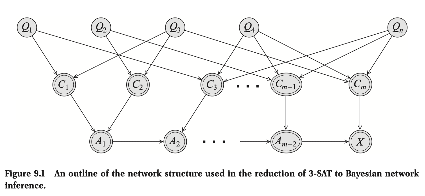
- re: (1), at first glance the treewidth of 3-SAT (clearly dependent on the structure of the - interaction) doesn't seem super insightful or intuitive, though we may count the statement "a 3-SAT problem gets exponentially harder as you increase the formula-treewidth" as progress.
- ... but even that wouldn't be an if and only if characterization of 3-SAT difficulty, because re: (2) there exist easy-in-practice 3-SAT problems that don't necessarily have bounded treewidth (i haven't read the link).
I would be interested in a similar analysis for more NP-complete problems known to have natural parameterized complexity characterization.
There is another interesting connection between computation and bounded treewidth: the control flow graphs of programs written in languages "without goto instructions" have uniformly bounded treewidth (e.g. <7 for goto-free C programs). This is due to Thorup (1998):
https://www.sciencedirect.com/science/article/pii/S0890540197926973
Combined with graphs algorithms for bounded treewidth graphs, this has apparently been used in the analysis of compiler optimization and program verification problems, see the recent reference:
https://dl.acm.org/doi/abs/10.1145/3622807
which also proves a similar bound for pathwidth.
Thanks for writing this up Dalcy!
My knowledge of computational complexity is unfortunately lacking. I too wonder to what degree the central definitions of the complexity classes truly reflect the deep algorithmic structures or perhaps are a rather coarse shadow of more complex invariants.
You mention treewidth - are there other quantities of similar importance?
I also wonder about treewidth. I looked up the definition on wikipedia but struggle to find a good intuitive story what it really measures. Do you have an intuition pump about treewidth you could share?
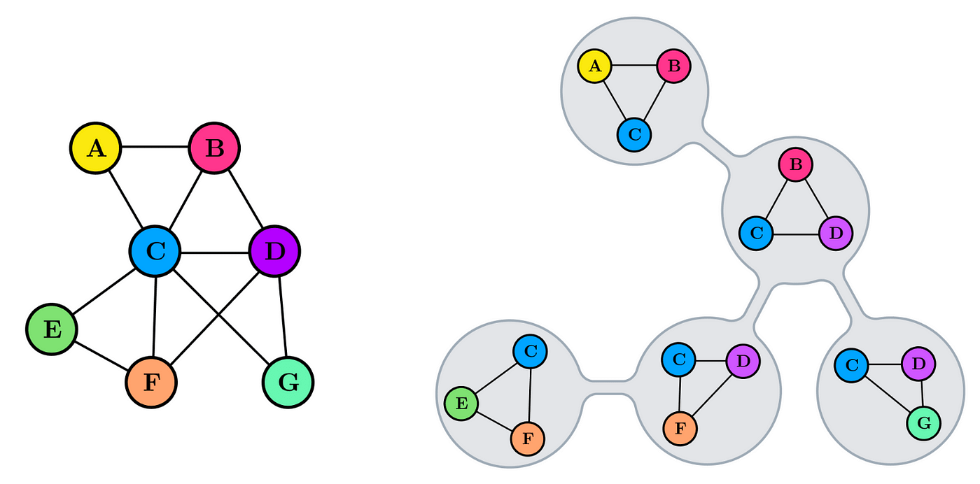
I like to think of treewidth in terms of its characterization from tree decomposition, a task where you find a clique tree (or junction tree) of an undirected graph.
Clique trees for an undirected graph is a tree such that:
- node of a tree corresponds to a clique of a graph
- maximal clique of a graph corresponds to a node of a tree
- given two adjacent tree nodes, the clique they correspond to inside the graph is separated given their intersection set (sepset)
You can check that these properties hold in the example below. I will also refer to nodes of a clique tree as 'cliques'. (image from here)
My intuition for the point of tree decompositions is that you want to coarsen the variables of a complicated graph so that they can be represented in a simpler form (tree), while ensuring the preservation of useful properties such as:
- how the sepset mediates (i.e. removing the sepset from the graph separates the variables associated with all of the nodes on one side of the tree with another) the two cliques in the original graph
- clique trees satisfy the running intersection property: if (the cliques corresponding to) the two nodes of a tree contain the same variable X, then X is also contained in (the cliques corresponding to) each and all of the intermediate nodes of the tree.
- Intuitively, information flow about a variable must connected, i.e. they can't suddenly disappear and reappear in the tree.
Of course tree decompositions aren't unique (image):
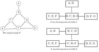
So we define .
- Intuitively, treewidths represent the degree to which nodes of a graph 'irreducibly interact with one another', if you really want to see the graph as a tree.
- e.g., the first clique tree of the image above is a suboptimal coarse graining in that it misleadingly characterizes as having a greater degree of 'irreducible interaction' among.
You mention treewidth - are there other quantities of similar importance?
I'm not familiar with any, though ChatGPT does give me some examples! copy-pasted below:
- Solution Size (k): The size of the solution or subset that we are trying to find. For example, in the k-Vertex Cover problem, k is the maximum size of the vertex cover. If k is small, the problem can be solved more efficiently.
- Treewidth (tw): A measure of how "tree-like" a graph is. Many hard graph problems become tractable when restricted to graphs of bounded treewidth. Algorithms that leverage treewidth often use dynamic programming on tree decompositions of the graph.
- Pathwidth (pw): Similar to treewidth but more restrictive, pathwidth measures how close a graph is to a path. Problems can be easier to solve on graphs with small pathwidth.
- Vertex Cover Number (vc): The size of the smallest vertex cover of the graph. This parameter is often used in graph problems where knowing a small vertex cover can simplify the problem.
- Clique Width (cw): A measure of the structural complexity of a graph. Bounded clique width can be used to design efficient algorithms for certain problems.
- Max Degree (Δ): The maximum degree of any vertex in the graph. Problems can sometimes be solved more efficiently when the maximum degree is small.
- Solution Depth (d): For tree-like or hierarchical structures, the depth of the solution tree or structure can be a useful parameter. This is often used in problems involving recursive or hierarchical decompositions.
- Branchwidth (bw): Similar to treewidth, branchwidth is another measure of how a graph can be decomposed. Many algorithms that work with treewidth also apply to branchwidth.
- Feedback Vertex Set (fvs): The size of the smallest set of vertices whose removal makes the graph acyclic. Problems can become easier on graphs with a small feedback vertex set.
- Feedback Edge Set (fes): Similar to feedback vertex set, but involves removing edges instead of vertices to make the graph acyclic.
- Modular Width: A parameter that measures the complexity of the modular decomposition of the graph. This can be used to simplify certain problems.
- Distance to Triviality: This measures how many modifications (like deletions or additions) are needed to convert the input into a simpler or more tractable instance. For example, distance to a clique, distance to a forest, or distance to an interval graph.
- Parameter for Specific Constraints: Sometimes, specific problems have unique natural parameters, like the number of constraints in a CSP (Constraint Satisfaction Problem), or the number of clauses in a SAT problem.
Tl;dr, While an algorithm's computational complexity may be exponential in general (worst-case), it is often possible to stratify its input via some dimension k that makes it polynomial for a fixed k, and only exponential in k. Conceptually, this quantity captures the core aspect of a problem's structure that makes specific instances of it 'harder' than others, often with intuitive interpretations.
Example: Bayesian Inference and Treewidth
One can easily prove exact inference (decision problem of: "is P(X)>0?") is NP-hard by encoding SAT-3 as a Bayes Net. Showing that it's NP is easy too.
Therefore, inference is NP-complete, implying that algorithms are worst-case exponential. But this can't be the typical case! Let's examine the example of a Bayes Net whose structure is a chain A⟶B⟶C⟶D, and say you want to compute the marginals P(D).
The Naive Algorithm for marginalization would be to literally multiply all the conditional probability distribution (CPD) tables for each of the Bayes Net's nodes, and sum over all the variables other than X. If we assume each variable has at most v values, then the computational complexity is exponential in the number of variables n.
But because of the factorization P(A,B,C,D)=P(A)P(B|A)P(C|B)P(D|C) due to the chain structure, we can shift the order of the sum around like this:
and now the sum can be done in O(nv2). Why?
So, at least for chains, inference can be done in linear time in input size.
The earlier NP-completeness result, remember, is a worst-case analysis that applies to all possible Bayes Nets, ignoring the possible structure in each instance that may make some easier to solve than the other.
Let's attempt a more fine complexity analysis by taking into account the structure of the Bayes Net provided, based on the chain example.
Intuitively, the relevant structure of the Bayes Net that determines the difficulty of marginalization is the 'degree of interaction' among the variables, since the complexity is exponential in the "maximum number of factors ever seen within a sum," which was 2 in the case of a chain.
How do we generalize this quantity to graphs other than chains?
Since we could've shuffled the order of the sums and products differently (which would still yield O(nv2) for chains, but for general graphs the exponent may change significantly), for a given graph we want to find the sum-shuffling-order that minimizes the number of factors ever seen within a sum, and call that number k, an invariant of the graph that captures the difficulty of inference — O(mvk)[1]
This is a graphical quantity of your graph called treewidth[2][3].
So, to sum up:
General Lesson
While I was studying basic computational complexity theory, I found myself skeptical of the value of various complexity classes, especially due to the classes being too coarse and not particularly exploiting the structures specific to the problem instance:
But while studying graphical models, I learned that, there are many more avenues of fine-grained complexity analyses (after the initial coarse classification) that may lend real insight to the problem's structure, such as parameterized complexity.
While many algorithms (e.g., those for NP-complete problems) are exponential (or more generally, superpolynomial) in input size in general (worst-case), there are natural problems whose input can be stratified via a parameter k - whose algorithms are polynomial in input size given a fixed k, and only exponential in k.
This is exciting from a conceptual perspective, because k then describes exactly what about the problem structure makes some instance of it harder or easier to solve, often with intuitive meanings - like treewidth!
Also, I suspect this may shed light on to what makes some NP-hardness results not really matter much in practice[4] - they don't matter because natural instances of the problem have low values of k. From this, one may conjecture that nature has low treewidth, thus agents like us can thrive and do Bayes.
m is the number of times the sum was performed. In the case of chains, this was simply n−1, thus O(nv2). I omitted m because it seemed like an irrelevant detail for conveying the overall lesson.
A graphical quantity of your undirected graph by turning all the directed edges of the Bayes Net to undirected ones.
Actually, k−1 is treewidth. Trees (which chains are an example of) have a treewidth of 1, thus k=2.
Among many other reasons also laid out in the link, such as use of approximations, randomization, and caring more about average / generic case complexity. My point may be considered an elaboration of the latter reason.