The central limit theorems all say that if you convolve stuff enough, and that stuff is sufficiently nice, the result will be a Gaussian distribution. How much is enough, and how nice is sufficient?
Identically-distributed distributions converge quickly
For many distributions , the repeated convolution looks Gaussian. The number of convolutions you need to look Gaussian depends on the shape of . This is the easiest variant of the central limit theorem: identically-distributed distributions.
The uniform distribution converges real quick:
The numbers on the x axis are increasing because the mean of is the sum of the means of and , so if we start with positive means, repeated convolutions shoot off into higher numbers. Similar for the variance - notice how the width starts as the difference between 1 and 2, but ends with differences in the tens. You can keep the location stationary under convolution by starting with a distribution centered at 0, but you can't keep the variance from increasing, because you can't have a variance of 0 (except in the limiting case).
Here's a more skewed distribution: beta(50, 1). beta(50, 1) is the probability distribution that represents knowing that a lake has bass and carp, but not how many of each, and then catching 49 bass in a row. It's fairly skewed! This time, after 30 convolutions, we're not quite Gaussian - the skew is still hanging around. But for a lot of real applications, I'd call the result "Gaussian enough".
A similar skew in the opposite direction, from the exponential distribution:
I was surprised to see the exponential distribution go into a Gaussian, because Wikipedia says that an exponential distribution with parameter goes into a gamma distribution with parameters gamma(, ) when you convolve it with itself times. But it turns out gamma() looks more and more Gaussian as goes up.
How about our ugly bimodal-uniform distribution?
It starts out rough and jagged, but already by 30 convolutions it's Gaussian.
And here's what it looks like to start with a Gaussian:
The red curve starts out the exact same as the black curve, then nothing happens because Gaussians stay Gaussian under self-convolution.
An easier way to measure Gaussianness (Gaussianity?)
We're going to want to look at many more distributions under convolutions and see how close they are to Gaussian, and these animations take a lot of space. We need a more compact way. So let's measure the kurtosis of the distributions, instead. The kurtosis is the fourth moment of a probability distribution; it describes the shape of the tails. All Gaussian distributions have kurtosis 3. There are other distributions with kurtosis 3, too, but they're not likely to be the result of a series of convolutions. So to check how close a distribution is to Gaussian, we can just check how far from 3 its kurtosis is.
We can chart the kurtosis as a function of how many convolutions have been done so far, for each of the five distributions above:
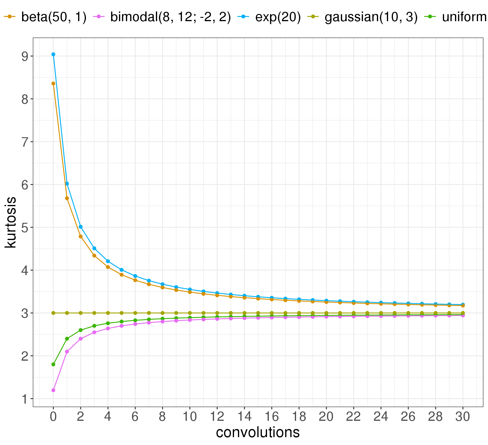
Notice: the distributions that have a harder time making it to Gaussian are the two skewed ones. It turns out the skew of a distribution goes a long way in determining how many convolutions you need to get Gaussian. Plotting the kurtosis at convolution 30 against the skew of the original distribution (before any convolutions) shows that skew matters a lot:
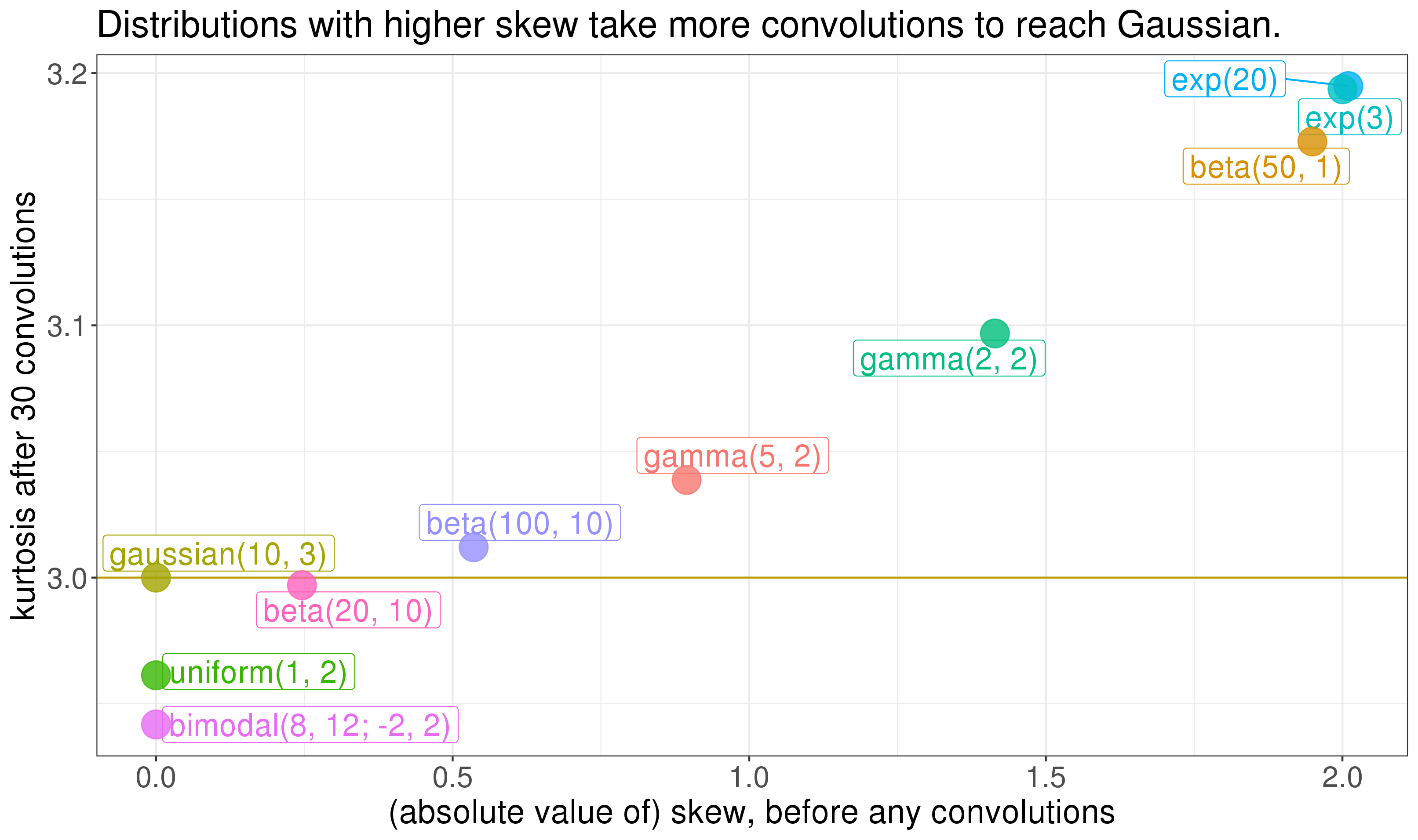
So the skew of the component distributions goes a long way in determining how quick their convolution gets Gaussian. The Berry-Esseen theorem is a central limit theorem that says something similar (but see this comment). So here's our first rule for eyeing things in the wild and trying to figure out whether the central limit theorem will apply well enough to get you a Gaussian distribution: how skewed are the input distributions? If they're viciously skewed, you should worry.
Non-identically-distributed distributions converge quickly too
In real problems, distributions won't be identically distributed. This is the interesting case. If instead of a single distribution convolved with itself, we take , then a version of the central limit theorem still applies - the result can still be Gaussian. So let's take a look.
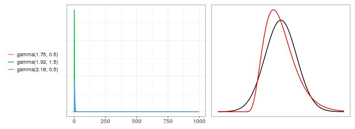
Here are three different Beta distributions, on the left, and on the right, their convolution, with same setup from the animations: red is the convolution, and black is the true Gaussian with the same mean and variance.
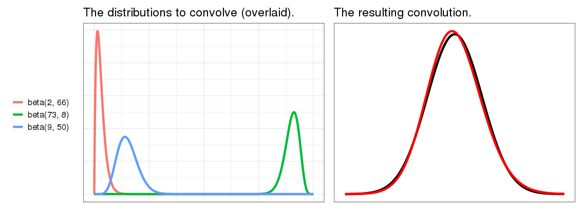
They've almost converged! This is a surprise. I really didn't expect as few as three distributions to convolve into this much of a Gaussian. On the other hand, these are pretty nice distributions - the blue and green look pretty Gaussian already. That's cheating. Let's try less nice distributions. We saw above that distributions with higher skew are less Gaussian after convolution, so let's crank up the skew. It's hard to get a good skewed Beta distribution, so let's use Gamma distributions instead.
Not Gaussian yet - the red convolution result line still looks Gamma-ish. But if we go up to a convolution of 30 gamma distributions this skewed...
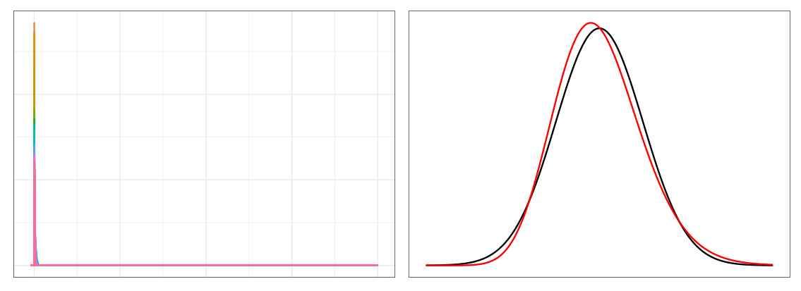
... already, we're pretty much Gaussian.
I'm really surprised by this. I started researching this expecting the central limit theorem convergence to fall apart, and require a lot of distributions, when the input distributions got this skewed. I would have guessed you needed to convolve hundreds to approach Gaussian. But at 30, they're already there! This helps explain how carefree people can be in assuming the CLT applies, sometimes even when they haven't looked at the distributions: convergence really doesn't take much.
To that point, skew and excess Kurtosis are just two of an infinite number of moments, so obviously they do not characterize the distribution. As someone else here suggested, one can look at the Fourier (or other) Transform, but then you are again left with evaluating the difference between two functions or distributions: knowing that the FT of a Gaussian is a Gaussian in its dual space doesn't help with "how close" a t-domain distribution F(t) is to a t-domain Gaussian G(t), you've just moved the problem into dual space.
We have a tendency to want to reduce an infinite dimensional question to a one dimensional answer. How about the L1 norm or the L2 norm of the difference? Well, the L2 norm is preserved under FT, so nothing is gained. Using the L1 norm would require some justification other than "it makes calculation easy".
So it really boils down to what question you are asking, what difference does the difference (between some function and the Gaussian) make? If being wrong (F(t) != G(t) for some t) leads to a loss of money, then use this as the "loss" function. If it is lives saved or lost use that loss function on the space of distributions. All such loss functions will look like an integral over the domain of L(F(t), G(t)). In this framework, there is no universal answer, but once you've decided what your loss function is and what your tolerance is you can now compute how many approximations it takes to get your loss below your tolerance.
Another way of looking at it is to understand what we are trying to compare the closeness of the test distribution to. It is not enough to say F(t) is this close to the Gaussian unless you can also tell me what it is not. (This is the "define a cat" problem for elementary school kids.) Is it not close to a Laplace distribution? How far away from Laplace is your test distribution compared to how far away it is from Gaussian? For these kinds of questions - where you want to distinguish between two (or more) possible candidate distributions - the Likelihood ratio is a useful metric.
Most data sceancetists and machine learning smiths I've worked with assume that in "big data" everything is going to be a normal distribution "because Central Limit Theorem". But they don't stop to check that their final distribution is actually Gaussian (they just calculate the mean and the variance and make all sorts of parametric assumptions and p-value type interpretations based on some z-score), much less whether the process that is supposed to give rise to the final distribution is one of sampling repeatedly from different distributions or can be genuinely modeled as convolutions.
One example: the distribution of coefficients in a Logistic model is assumed (by all I've spoken to) to be Gaussian ("It is peaked in the middle and tails off to the ends."). Analysis shows it to be closer to Laplace, and one can model the regression process itself as a diffusion equation in one dimension, whose solution is ... Laplace!
I can provide an additional example, this time of a sampling process, where one is sampling from hundreds of distributions of different sizes (or weights), most of which are close to Gaussian. The distribution of the sum is once again, Laplace! With the right assumptions, one can mathematically show how you get Laplace from Gaussians.