This post was written as part of the AISC under supervision of John Wentworth. I started my PhD simultaneously with this project and admit that I underestimated the necessary effort to excel at both. I still had a great time, learned a lot and met a bunch of interesting people. I never hit upon the "one cool thing", but I hope this post still has some useful takeaways.
I would like to thank John Wentworth for his supervision and Lucius Bushnaq for our brainstorming sessions. I would also like to thank the AISC team for organizing the event. Finally, I'd like to thank Lauro Langosco for recommending AISC to me.
Consider some agent maximizing some utility. We usually model this agent to be in some environment. It can be reasonable to assume that the environment we find ourselves in is noisy. There are two (mostly) equivalent ways this can happen: either our observations contain some noise, or our actions are performed noisily. Even if the environment is not noisy we might still gain some useful properties from training an agent with (some kinds of) noise. There is mild evidence suggesting it helps with robustness, see e.g. Open AI's robot hand or this paper. I want to investigate a particular formalism of how to treat noise. From this formalism I hope to gain - A definition / understanding of noise resistance - Protection against distributional shifts - Better generalization - Other theoretical insights
How I got here
The project started with the hope to expand the idea of Utility Maximization as compression. This is related to the Telephone Theorem and the Generalized Heat Engine. While exploring these ideas I played around with various models, and particularly focused on ones where compression works nicely. Not unsurprisingly boolean functions were particularly insightful, as they are both easy to do explicit calculations with and more easily relate to compression. This lead me to the theory of boolean functions and noise sensitivity, which I then viewed as a utility function, although many interpretations are possible / useful.
Formal setup
Consider some finite space A. We consider two classes of functions: 1. Boolean functions taking bits as input and returning bits as output i.e. u:{−1,1}A→{−1,1}. 2. Generalized boolean functions which instead returns a real number i.e. u:{−1,1}A→R.
In the rest of the post I will not always specify the type of Boolean function, it should hopefully be clear from context. Either way, we can think of {−1,1}A as the space of actions we can take, sub-actions for a single actions or multiple sub-agents voting for different actions.
Let us start by consider the following maximization problem:
maxω∈ΩE[u(ωε)]=maxω¯¯¯u(ω),
where ωε is the random variable where each bit of ω is resampled with probability ε, i.e. we expect the environment to augment our chosen ω with a bit of noise. We can choose a different amount of noise for every bit, the following theory would still hold, but it would be more tedious to write it out. Some questions that now naturally arise might be: - Can we naturally represent ¯¯¯u? - How much does the optimal ω change? - How good is the optimal ω∗=argmaxω¯¯¯u(ω) for u?
It is natural to think of ¯¯¯u as a smoothed version of u. Unless the function is constant, the maximum will be suppressed and the minimum will be increased.
To help us guide our thinking about the above questions we introduce the following definitions. These are noise sensitivity and noise stability. They won't perfectly map onto the problem in the way that I have set it up, but they will still be conceptually useful. As we will see later, these definitions also naturally expand. In the following definitions we consider the uniform distribution over all bit configurations.
We call a family un:{−1,1}n→{−1,1} noise sensitive if
limn→∞E[un(ω)un(ωε)]−E[un(ω)]2=0,
for all ε>0. In other words it is noise sensitive if the random variables un(ω) and un(ωε) totally decorrelate.
On the other hand, we call a sequence noise stable if
limε→0supnP[un(ω)≠un(ωε)]=0.
This intuitively means that the random perturbation has no effect on the function in the limit.
You can check that a sequence is both noise sensitive and stable if and only if the $u_n$'s become almost surely deterministic in the limit.
Examples
Examples of noise stable function classes are majority, i.e. un evaluates to 1 if there are more 1's and to -1 else, and dictator: i.e. a single bit decides the outcome.
Noise sensitive functions include the parity of bits, that is the product of all input bits. And also the iterated 3-majority: for n=3k we group the bits into 3's and then evaluate the majority for each group. We repeat this process until there is a single bit left.
Noisy utility maximization
To get a shift in perspective we can use a common tool, which ubiquitous throughout mathematics, the Fourier transform. Intuitively it shifts our view from the current domain to a frequency domain. For discrete systems this is basically a change of basis for a well chosen orthonormal basis. So let us choose a particularly useful basis:
(χS)S⊂AχS(ω)=∏i∈Sωi.
Note that this can also be seen as a polynomial representation. For every χS we have E[χS]=0 and Var(χS)=1. For a given S this can be thought of as the S-parity. This allows us to deconstruct a given u as follows
^u(S)=E[u⋅χS].
We think of larger sets S corresponding to higher frequencies. Note that when S=∅, then we simply get the expected value. We can then reconstruct u as follows
u(ω)=∑S^u(S)χS(ω).
Why is this useful? We can more easily show things about the χS's then all of u at the same time. In particular, it is easily shown that
E[χS(ωε)]=χS(ω)(1−ε)|S|.
In other words the higher frequencies get dampened. This is a stronger statement than appears on the surface. We can see that this allows us to write ¯¯¯u as follows:
¯¯¯u(ω)=∑S^u(S)χS(ω)(1−ε)|S|.
Now consider the following theorems.
We define Eu(m):=∑S:|S|=m^u(S)2 to be the energy at frequency m.
A sequence of boolean functions {fn}:{±1}mn→{0,1} is noise sensitive if and only if ∀k≥1 we find:
∑S:|S|≤k^fn(S)2=k∑m=1Efn(m)→0
as n→∞.
Similarly we find
A sequence is noise stable if and only if ∀ε>0 there exists a k such that for all n
∞∑m=kEfn(m)<ε.
The dampening effect from above shows that
E¯¯¯u(m)=(1−ε)2mEu(m).
This means that the function ¯¯¯u=E[u(⋅ε)] is automatically noise stable (if the energies at higher frequencies grow sub-exponentially).
Furthermore, we can take this as the definition of noise sensitivity / stability for general boolean functions.
These theorems also tells us that we can perform what looks like a lossy compression of u. We simply cut off all high frequency elements, as we might do in jpeg compression. This should still be good approximation of u as these terms get arbitrarily small in the face of noise.
The biggest issue with this approach in practice is that it is computationally very costly. Iterating through all subsets up to some size n is of order O(2n).
Notes & Outlook
Gaussian extension
The first way to expand these ideas is to generalize to functions with more general domains. If you interpret a coin flip as a 0d Gaussian random variable (which might or might not be reasonable), a natural extension might be Gaussian processes. In this paper Gaussians are used to approximate binary random variables. They are also especially nice as there is an inherent connection to both the Fourier transform and uncertainty. Furthermore, as in the telephone theorem we have Driscoll's 0-1 law for Gaussian processes, saying that globally certain statistics always hold or never hold.
Subagents
In John's post Why subagents? he argues that sub-agents generally describe many systems better than single agents would. In particular things like the stock market or even individual humans have no utility function. We can extend this description with boolean functions. A boolean function f can be interpreted as a voting system between two or more outcomes / actions. Each bit is interpreted as a vote from a single sub-agent. By Arrow's impossibility theorem however, we know that if the voting system is rational (for some reasonable definition) then our boolean function f must be the dictator function - i.e. decided by a single bit / voter. This seems like some mild evidence against certain kinds of subagents.
You might argue that humans and stock markets are just mostly rational and so Arrow's theorem doesn't apply. However, his theorem can be strengthened to basically say that if we are irrational about ε of the time, then f has to be ε-close to the dictator function, in some precise sense. So if we believe humans are mostly rational, then we also have to accept that we are mostly agents. This does not rule out things like Kelly-betting or liquid democracy to gain consensus, as they are not captured by the boolean framework.
Qubit extension
We could use qubits as inputs to our functions, instead of traditional bits. To massively oversimplify, the extension to the quantum regime allows bits some limited communication. It is shown that all sorts of problems have more satisfying solutions in the quantum realm. For example, when playing the prisoners dilemma with entangled qubits the optimal strategy leads to cooperation instead of defection[1]. We can also get around Arrow's impossibility theorem when voting with qubits. In particular this means if subagents can share information (in the way entangled bits can) then the dictatorship is not the only rational voting system. Some limited work has already been done for more general boolean function, but it does not yet seem satisfactory.
Noise and Flatness
There are two (related) connections that I see. The first is to the Telephone Theorem which states that in the world only certain kinds of information can travel "far". In some sense the details are lost in the noise and important summary statistics survive arbitrarily long. In other words, optimizing with noise is similar to optimizing at a distance. The other is the relation between generalized solutions and "basin flatness". In the post Information loss --> Basin Flatness the shape of the loss function is heuristically related generalization. Low frequency terms dominating the the loss function locally (in its Fourier transform) might be a useful proxy for this. Low frequency terms dominating also exactly relates to noise stability. Both of these ideas show that in some sense the "important" optimization is along a low-dimensional manifold in our parameter space.
The code for the following two subsections should hopefully be upload to git soon.
Computation of Energies and the noisy regime
Consider the following toy scenario. We want to build a bridge from left to right. We only get reward if the bridge is completed, but every extra bit we use costs us some utility. Furthermore, we live in a noisy world where bits are randomly flipped. If our utility function is well chosen the optimal bridge might look as follows: After applying some noise the bridge gets modified as such:
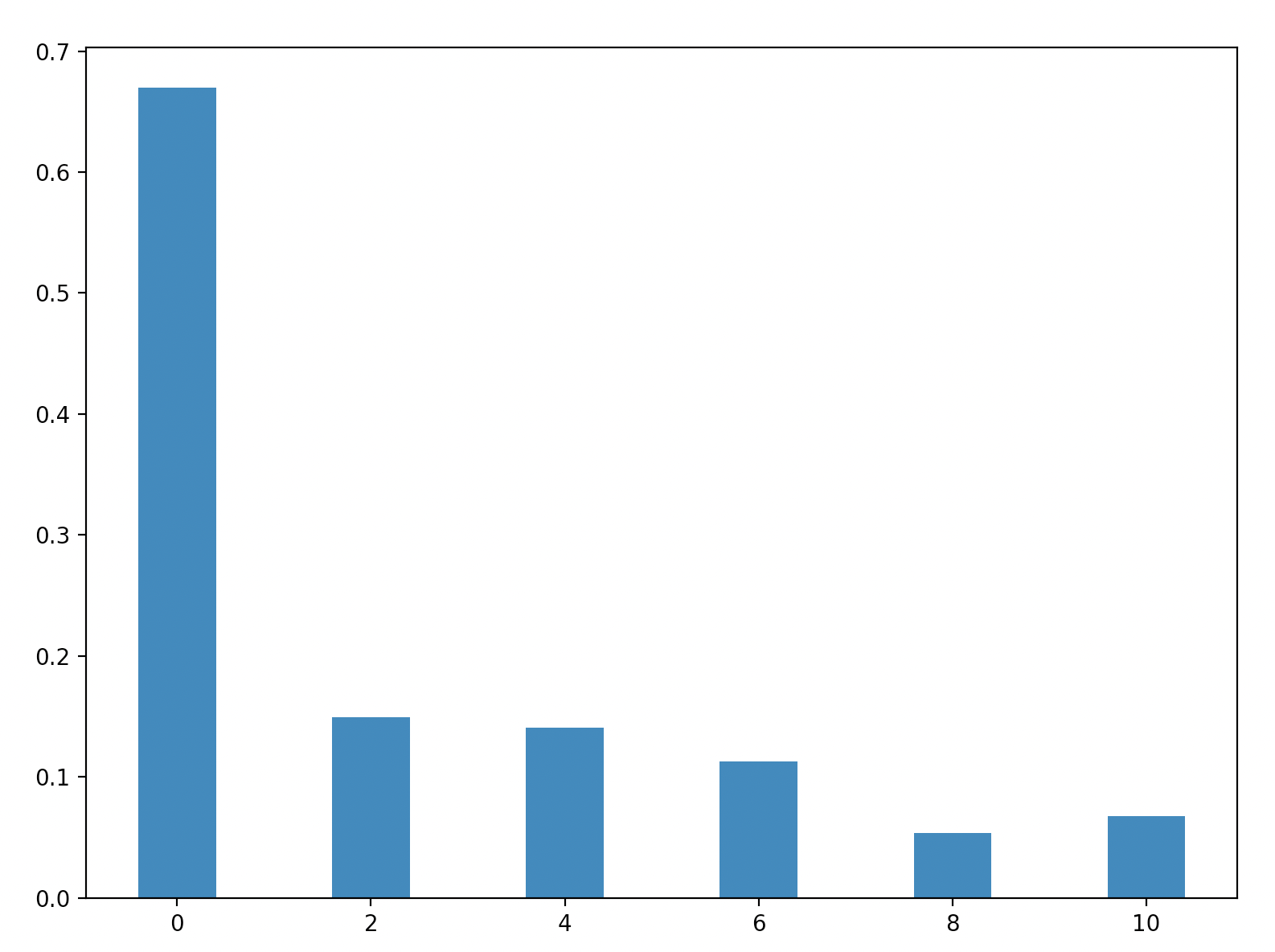
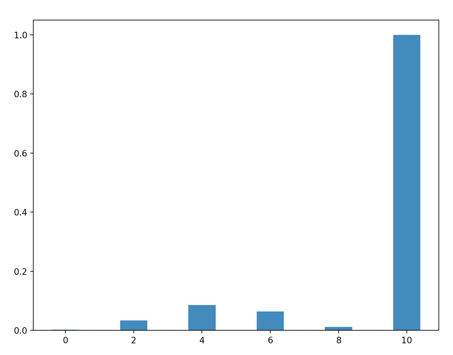
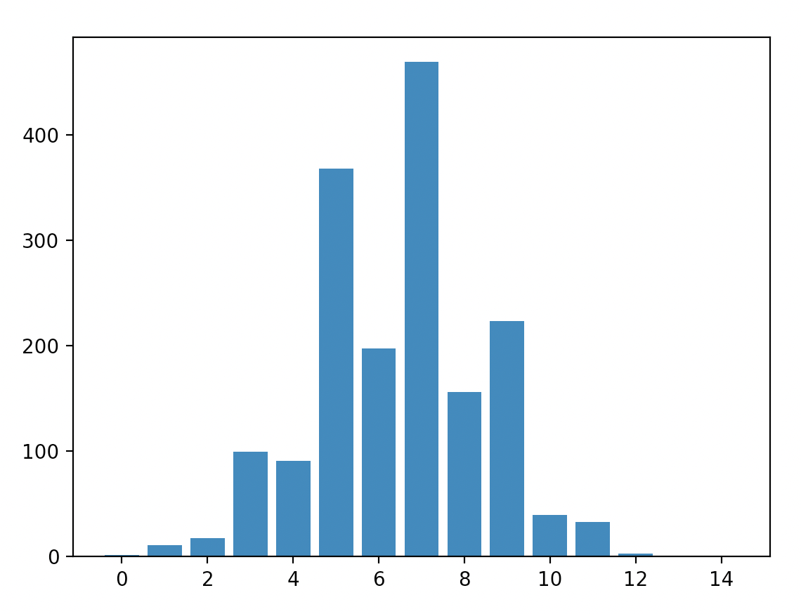
Using the equations for energy above to directly calculate the different energies. To do this deterministically would not be feasible as we would have to iterate over sets of subsets. The first approach I tried was to use Monte Carlo simulations instead. We get the following results:
Majority:
Parity:
Bridge 3x5 setup:
We can tell that in my probabilistic simulation of the energies there is a significant amount of variance. Since we are squaring the terms this leads to bias. This can be seen most easily be seen in the parity - only the final column should have any energy, yet there are positive energies in 2, 4, 6 and 8 in this simulation.
In this current version the energies for the 3x5 bridge is probably just dominated by noise.
Efficient computation
There is a better method to calculate the energies of a function using an inverse problem. By applying some of the equations discussed above we find that
Covω(u(ω),u(ωε))=n∑i=1Eu(i)(1−ε)i.
We can of course estimate these covariances directly given the utility function u. If we do this for n different values of ε we get a linear system where we can solve for x. In particular we get the linear system
Ax=b
where A is a design matrix with entries aij=(1−εi)j and b is given by the corresponding covariances bi=Covω(u(ω),u(ωεi)). We solve for x.
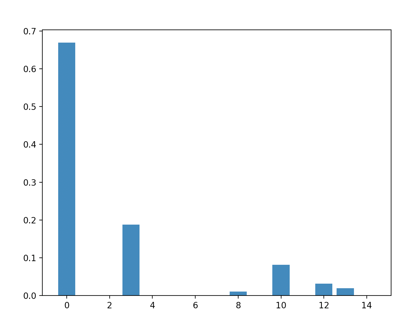
This set up mostly buys us speed. By the nature of inverse problems however, the solution is very sensitive with respect to A and b. Thus the covariances have to be estimated with a lot of accuracy. We get the following.
Majority with 15 bits:
Parity with 15 bits:
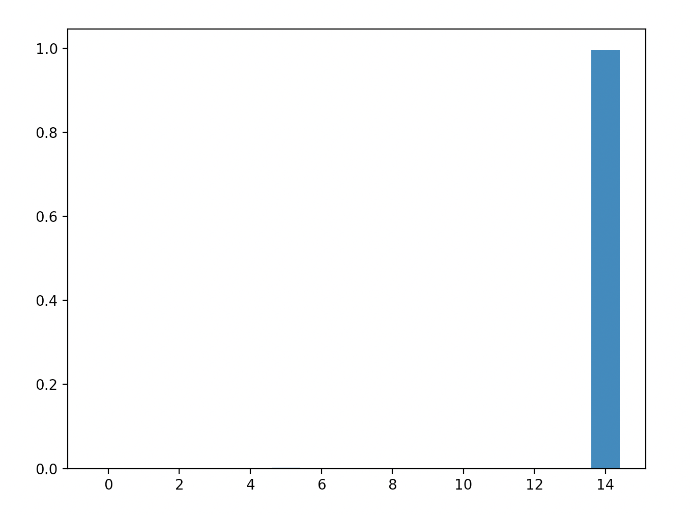
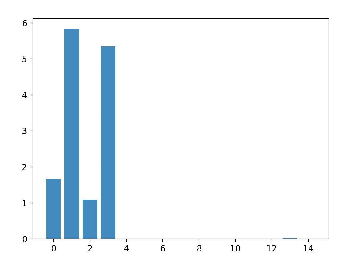
Bridge with 3x5 setup:
If we call the bridge utility function u, then we can run the energy code again with the utility function ¯¯¯u. We get the following: As we can see the energies are concentrated at the lowest energy level (though this is definitely a crude estimation).
This post was written as part of the AISC under supervision of John Wentworth. I started my PhD simultaneously with this project and admit that I underestimated the necessary effort to excel at both. I still had a great time, learned a lot and met a bunch of interesting people. I never hit upon the "one cool thing", but I hope this post still has some useful takeaways.
I would like to thank John Wentworth for his supervision and Lucius Bushnaq for our brainstorming sessions. I would also like to thank the AISC team for organizing the event. Finally, I'd like to thank Lauro Langosco for recommending AISC to me.
Consider some agent maximizing some utility. We usually model this agent to be in some environment. It can be reasonable to assume that the environment we find ourselves in is noisy. There are two (mostly) equivalent ways this can happen: either our observations contain some noise, or our actions are performed noisily.
Even if the environment is not noisy we might still gain some useful properties from training an agent with (some kinds of) noise. There is mild evidence suggesting it helps with robustness, see e.g. Open AI's robot hand or this paper. I want to investigate a particular formalism of how to treat noise. From this formalism I hope to gain
- A definition / understanding of noise resistance
- Protection against distributional shifts
- Better generalization
- Other theoretical insights
How I got here
The project started with the hope to expand the idea of Utility Maximization as compression. This is related to the Telephone Theorem and the Generalized Heat Engine. While exploring these ideas I played around with various models, and particularly focused on ones where compression works nicely. Not unsurprisingly boolean functions were particularly insightful, as they are both easy to do explicit calculations with and more easily relate to compression. This lead me to the theory of boolean functions and noise sensitivity, which I then viewed as a utility function, although many interpretations are possible / useful.
Formal setup
Consider some finite space A. We consider two classes of functions:
1. Boolean functions taking bits as input and returning bits as output i.e. u:{−1,1}A→{−1,1}.
2. Generalized boolean functions which instead returns a real number i.e. u:{−1,1}A→R.
In the rest of the post I will not always specify the type of Boolean function, it should hopefully be clear from context. Either way, we can think of {−1,1}A as the space of actions we can take, sub-actions for a single actions or multiple sub-agents voting for different actions.
Let us start by consider the following maximization problem:
maxω∈ΩE[u(ωε)]=maxω¯¯¯u(ω),where ωε is the random variable where each bit of ω is resampled with probability ε, i.e. we expect the environment to augment our chosen ω with a bit of noise. We can choose a different amount of noise for every bit, the following theory would still hold, but it would be more tedious to write it out.
Some questions that now naturally arise might be:
- Can we naturally represent ¯¯¯u?
- How much does the optimal ω change?
- How good is the optimal ω∗=argmaxω¯¯¯u(ω) for u?
It is natural to think of ¯¯¯u as a smoothed version of u. Unless the function is constant, the maximum will be suppressed and the minimum will be increased.
To help us guide our thinking about the above questions we introduce the following definitions. These are noise sensitivity and noise stability. They won't perfectly map onto the problem in the way that I have set it up, but they will still be conceptually useful. As we will see later, these definitions also naturally expand. In the following definitions we consider the uniform distribution over all bit configurations.
You can check that a sequence is both noise sensitive and stable if and only if the $u_n$'s become almost surely deterministic in the limit.
Examples
Examples of noise stable function classes are majority, i.e. un evaluates to 1 if there are more 1's and to -1 else, and dictator: i.e. a single bit decides the outcome.
Noise sensitive functions include the parity of bits, that is the product of all input bits. And also the iterated 3-majority: for n=3k we group the bits into 3's and then evaluate the majority for each group. We repeat this process until there is a single bit left.
Noisy utility maximization
To get a shift in perspective we can use a common tool, which ubiquitous throughout mathematics, the Fourier transform. Intuitively it shifts our view from the current domain to a frequency domain. For discrete systems this is basically a change of basis for a well chosen orthonormal basis. So let us choose a particularly useful basis:
(χS)S⊂AχS(ω)=∏i∈Sωi.Note that this can also be seen as a polynomial representation. For every χS we have E[χS]=0 and Var(χS)=1. For a given S this can be thought of as the S-parity. This allows us to deconstruct a given u as follows
^u(S)=E[u⋅χS].We think of larger sets S corresponding to higher frequencies. Note that when S=∅, then we simply get the expected value. We can then reconstruct u as follows
u(ω)=∑S^u(S)χS(ω).Why is this useful? We can more easily show things about the χS's then all of u at the same time. In particular, it is easily shown that
E[χS(ωε)]=χS(ω)(1−ε)|S|.In other words the higher frequencies get dampened. This is a stronger statement than appears on the surface. We can see that this allows us to write ¯¯¯u as follows:
¯¯¯u(ω)=∑S^u(S)χS(ω)(1−ε)|S|.Now consider the following theorems.
We define Eu(m):=∑S:|S|=m^u(S)2 to be the energy at frequency m.
Similarly we find
The dampening effect from above shows that
E¯¯¯u(m)=(1−ε)2mEu(m).This means that the function ¯¯¯u=E[u(⋅ε)] is automatically noise stable (if the energies at higher frequencies grow sub-exponentially).
Furthermore, we can take this as the definition of noise sensitivity / stability for general boolean functions.
These theorems also tells us that we can perform what looks like a lossy compression of u. We simply cut off all high frequency elements, as we might do in jpeg compression. This should still be good approximation of u as these terms get arbitrarily small in the face of noise.
The biggest issue with this approach in practice is that it is computationally very costly. Iterating through all subsets up to some size n is of order O(2n).
Notes & Outlook
Gaussian extension
The first way to expand these ideas is to generalize to functions with more general domains. If you interpret a coin flip as a 0d Gaussian random variable (which might or might not be reasonable), a natural extension might be Gaussian processes. In this paper Gaussians are used to approximate binary random variables. They are also especially nice as there is an inherent connection to both the Fourier transform and uncertainty. Furthermore, as in the telephone theorem we have Driscoll's 0-1 law for Gaussian processes, saying that globally certain statistics always hold or never hold.
Subagents
In John's post Why subagents? he argues that sub-agents generally describe many systems better than single agents would. In particular things like the stock market or even individual humans have no utility function. We can extend this description with boolean functions. A boolean function f can be interpreted as a voting system between two or more outcomes / actions. Each bit is interpreted as a vote from a single sub-agent. By Arrow's impossibility theorem however, we know that if the voting system is rational (for some reasonable definition) then our boolean function f must be the dictator function - i.e. decided by a single bit / voter. This seems like some mild evidence against certain kinds of subagents.
You might argue that humans and stock markets are just mostly rational and so Arrow's theorem doesn't apply. However, his theorem can be strengthened to basically say that if we are irrational about ε of the time, then f has to be ε-close to the dictator function, in some precise sense. So if we believe humans are mostly rational, then we also have to accept that we are mostly agents.
This does not rule out things like Kelly-betting or liquid democracy to gain consensus, as they are not captured by the boolean framework.
Qubit extension
We could use qubits as inputs to our functions, instead of traditional bits. To massively oversimplify, the extension to the quantum regime allows bits some limited communication. It is shown that all sorts of problems have more satisfying solutions in the quantum realm. For example, when playing the prisoners dilemma with entangled qubits the optimal strategy leads to cooperation instead of defection[1]. We can also get around Arrow's impossibility theorem when voting with qubits. In particular this means if subagents can share information (in the way entangled bits can) then the dictatorship is not the only rational voting system. Some limited work has already been done for more general boolean function, but it does not yet seem satisfactory.
Noise and Flatness
There are two (related) connections that I see. The first is to the Telephone Theorem which states that in the world only certain kinds of information can travel "far". In some sense the details are lost in the noise and important summary statistics survive arbitrarily long. In other words, optimizing with noise is similar to optimizing at a distance.
The other is the relation between generalized solutions and "basin flatness". In the post Information loss --> Basin Flatness the shape of the loss function is heuristically related generalization. Low frequency terms dominating the the loss function locally (in its Fourier transform) might be a useful proxy for this. Low frequency terms dominating also exactly relates to noise stability.
Both of these ideas show that in some sense the "important" optimization is along a low-dimensional manifold in our parameter space.
Some More References
Boolean Function Survey by Ryan O’Donnell
Noise stability of functions with low influences
Noise stability of boolean functions
Appendix
The code for the following two subsections should hopefully be upload to git soon.
Computation of Energies and the noisy regime
Consider the following toy scenario. We want to build a bridge from left to right. We only get reward if the bridge is completed, but every extra bit we use costs us some utility. Furthermore, we live in a noisy world where bits are randomly flipped. If our utility function is well chosen the optimal bridge might look as follows:


After applying some noise the bridge gets modified as such:
Using the equations for energy above to directly calculate the different energies. To do this deterministically would not be feasible as we would have to iterate over sets of subsets. The first approach I tried was to use Monte Carlo simulations instead. We get the following results:
Majority:
Parity:
Bridge 3x5 setup:
We can tell that in my probabilistic simulation of the energies there is a significant amount of variance. Since we are squaring the terms this leads to bias. This can be seen most easily be seen in the parity - only the final column should have any energy, yet there are positive energies in 2, 4, 6 and 8 in this simulation.
In this current version the energies for the 3x5 bridge is probably just dominated by noise.
Efficient computation
There is a better method to calculate the energies of a function using an inverse problem. By applying some of the equations discussed above we find that
Covω(u(ω),u(ωε))=n∑i=1Eu(i)(1−ε)i.We can of course estimate these covariances directly given the utility function u. If we do this for n different values of ε we get a linear system where we can solve for x. In particular we get the linear system
Ax=bwhere A is a design matrix with entries aij=(1−εi)j and b is given by the corresponding covariances bi=Covω(u(ω),u(ωεi)). We solve for x.
This set up mostly buys us speed. By the nature of inverse problems however, the solution is very sensitive with respect to A and b. Thus the covariances have to be estimated with a lot of accuracy. We get the following.
Majority with 15 bits:
Parity with 15 bits:
Bridge with 3x5 setup:
If we call the bridge utility function u, then we can run the energy code again with the utility function ¯¯¯u. We get the following:
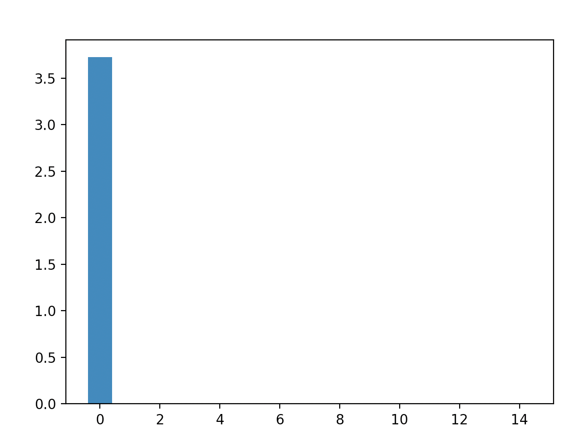
As we can see the energies are concentrated at the lowest energy level (though this is definitely a crude estimation).
More precisely, it unlocks new strategies that preempt the opponents move.