The critical insight is that this is not always the case!

Let's call two graphs I-equivalent if their set of independencies (implied by d-separation) are identical. A theorem of Bayes Nets say that two graphs are I-equivalent if they have the same skeleton and the same set of immoralities.

This last constraint, plus the constraint that the graph must be acyclic, allows some arrow directions to be identified - namely, across all I-equivalent graphs that are the perfect map of a distribution, some of the edges have identical directions assigned to them.

The IC algorithm (Verma & Pearl, 1990) for finding perfect maps (hence temporal direction) is exactly about exploiting these conditions to orient as many of the edges as possible:

More intuitively, (Verma & Pearl, 1992) and (Meek, 1995) together shows that the following four rules are necessary and sufficient operations to maximally orient the graph according to the I-equivalence (+ acyclicity) constraint:

Anyone interested in further detail should consult Pearl's Causality Ch 2. Note that for some reason Ch 2 is the only chapter in the book where Pearl talks about Causal Discovery (i.e. inferring time from observational distribution) and the rest of the book is all about Causal Inference (i.e. inferring causal effect from (partially) known causal structure).

The Metaphysical Structure of Pearl's Theory of Time

Epistemic status: metaphysics

I was reading Factored Space Models (previously, Finite Factored Sets) and was trying to understand in what sense it was a Theory of Time.

Scott Garrabrant says "[The Pearlian Theory of Time] ... is the best thing to happen to our understanding of time since Einstein". I read Pearl's book on Causality^[1], and while there's math, this metaphysical connection that Scott seems to make isn't really explicated. Timeless Causality and Timeless Physics is the only place I saw this view explained explicitly, but not at the level of math / language used in Pearl's book.

Here is my attempt at explicitly writing down what all of these views are pointing at (in a more rigorous language)—the core of the Pearlian Theory of Time, and in what sense FSM shares the same structure.

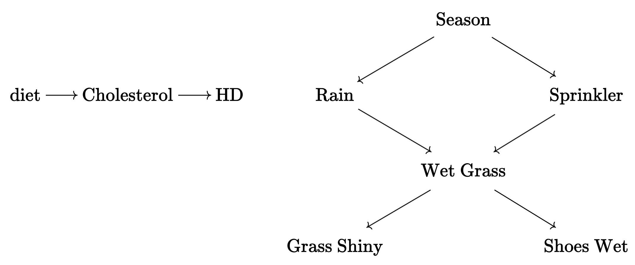
Causality leave a shadow of conditional independence relationships over the observational distribution. Here's an explanation providing the core intuition:

1. Suppose you represent the ground truth structure of [causality / determination] of the world via a Structural Causal Model over some variables, a very reasonable choice. Then, as you go down the Pearlian Rung: SCM $\to$^[2] Causal Bayes Net $\to$^[3] Bayes Net, theorems guarantee that the Bayes Net is still Markovian wrt the observational distribution.
   1. (Read Timeless Causality for an intuitive example.)
2. Causal Discovery then (at least in this example) reduces to inferring the equation assignment directions of the SCM, given only the observational distribution.
3. The earlier result guarantees that all you have to do is find a Bayes Net that is Markovian wrt the observational distribution. Alongside the faithfulness assumption, this thus reduces to finding a Bayes Net structure G whose set of independencies (implied by d-separation) are identical to that of P (or, finding the Perfect Map of a distribution^[4]).
4. Then, at least some of the edges of the Perfect Map will have its directions nailed down by the conditional independence relations.

The metaphysical claim is that, this direction is the definition of time^[5], morally so, based on the intuition provided by the example above.

So, the Pearlian Theory of Time is the claim that Time is the partial order over the variables of a Bayes Net corresponding to the perfect map of a distribution.

Abstracting away, the structure of any Theory of Time is then to:

1. find a mathematical structure [in the Pearlian Theory of Time, a Bayes Net]
2. ... that has gadgets [d-separation]
3. ... that are, in some sense, "equivalent" [soundness & completeness] to the conditional independence relations of the distribution the structure is modeling
4. ... while containing a notion of order [parenthood relationship of nodes in a Bayes Net]
5. ... while this order induced from the gadget coinciding to that of d-separation [trivially so here, because we're talking about Bayes Nets and d-separation] such that it captures the earlier example which provided the core intuition behind our Theory of Time.

This is exactly what Factored Space Model does:

1. find a mathematical structure [Factored Space Model]
2. ... that has gadgets [structural independence]
3. ... that are, in some sense, "equivalent" [soundness & completeness] to the conditional independence relations of the distribution the structure is modeling
4. ... while containing a notion of order [preorder relation induced by the subset relationship of the History]
5. ... while this order induced from the gadget coinciding to that of d-separation [by a theorem of FSM] such that it captures the earlier example which provided the core intuition behind our Theory of Time.
6. while, additionally, generalizing the scope of our Theory of Time from [variables that appear in the Bayes Net] to [any variables defined over the factored space].

... thus justifying calling FSM a Theory of Time in the same spirit that Pearlian Causal Discovery is a Theory of Time.

1. ^{^}

   Chapter 2, specifically, which is about Causal Discovery. All the other chapters are mostly irrelevant for this purpose.

2. ^{^}

   By (1) making a graph with edge direction corresponding to equation assignment direction, (2) pushforwarding uncertainties to endogenous variables, and (3) letting interventional distributions be defined by the truncated factorization formula.

3. ^{^}

   By (1) forgetting the causal semantics, i.e. no longer associating the graph with all the interventional distributions, and only the no intervention observational distribution.

4. ^{^}

   This shortform answers this question I had.

5. ^{^}

   Pearl comes very close. In his Temporal Bias Conjecture (2.8.2):

   "In most natural phenomenon, the physical time coincides with at least one statistical time."

   (where statistical time refers to the aforementioned direction.)

   But doesn't go as far as this ought to be the definition of Time.

The grinding inevitability is not a pressure on you from the outside, but a pressure from you, towards the world. This type of determination is the feeling of being an agent with desires and preferences. You are the unstoppable force, moving towards the things you care about, not because you have to but simply because that’s what it means to care. 

I think this is probably one of my favorite quotes of all time. I translated it to Korean (with somewhat major stylistic changes) with the help of ChatGPT:

의지(意志)라 함은,
하나의 인간으로서,
멈출 수 없는 힘으로 자신이 중요히 여기는 것들을 향해 나아가는 것.

이를 따르는 갈아붙이는 듯한 필연성은,
외부에서 자신을 압박하는 힘이 아닌,
스스로가 세상을 향해 내보내는 압력임을.

해야 해서가 아니라,
단지 그것이 무언가를 소중히 여긴다는 뜻이기 때문에.

https://www.lesswrong.com/posts/KcvJXhKqx4itFNWty/k-complexity-is-silly-use-cross-entropy-instead

The K-complexity of a function is the length of its shortest code. But having many many codes is another way to be simple! Example: gauge symmetries in physics. Correcting for length-weighted code frequency, we get an empirically better simplicity measure: cross-entropy.

However:

[this] is a well-known notion in algorithmic information theory, and differs from K-complexity by at most a constant

Epistemic status: literal shower thoughts, perhaps obvious in retrospect, but was a small insight to me.

I’ve been thinking about: “what proof strategies could prove structural selection theorems, and not just behavioral selection theorems?”

Typical examples of selection theorems in my mind are: coherence theorems, good regulator theorem, causal good regulator theorem.

• Coherence theorem: Given an agent satisfying some axioms, we can observe their behavior in various conditions and construct $U$, and then the agent’s behavior is equivalent to a system that is maximizing $U$.
  • Says nothing about whether the agent internally constructs $U$ and uses them.
• (Little Less Silly version of the) Good regulator theorem: A regulator $R$ that minimizes the entropy of a system variable $S$ (where there is an environment variable $X$ upstream of both $R$ and $S$) without unnecessary noise (hence deterministic) is behaviorally equivalent to a deterministic function of $S$ (despite being a function of $X$).
  • Says nothing about whether $R$ actually internally reconstructs $S$ and uses it to produce its output.
• Causal good regulator theorem (summary): Given an agent achieving low regret across various environment perturbations, we can observe their behavior in specific perturbed-environments, and construct $G^{\prime }$ that is very similar to the true environment $G$. Then argue: “hence the agent must have something internally isomorphic to $G$”. Which is true, but …
  • says nothing about whether the agent actually uses those internal isomorphic-to-$G$ structures in the causal history of computing its output.

And I got stuck here wondering, man, how do I ever prove anything structural.

Then I considered some theorems that, if you squint really really hard, could also be framed in the selection theorem language in a very broad sense:

• SLT: Systems selected to get low loss are likely to be in a degenerate part of the loss landscape.^[1]
  • Says something about structure: by assuming the system to be a parameterized statistical model, it says the parameters satisfy certain conditions like degeneracy (which further implies e.g., modularity).

This made me realize that to prove selection theorems on structural properties of agents, you should obviously give more mathematical structure to the “agent” in the first place:

• SLT represents a system as a parameterized function - very rich!
• In coherence theorem, the agent is just a single node that outputs decision given lotteries. In the good regulator theorem and the causal good regulator theorem, the agent is literally just a single node in a Bayes Net - very impoverished!

And recall, we actually have an agent foundations style selection theorem that does prove something structural about agent internals by giving more mathematical structure to the agent:

• Gooder regulator theorem: A regulator is now two nodes instead of one, but the latter-in-time node gets an additional information about the choice of “game” it is being played against (thus the former node acts as a sort of information bottleneck). Then, given that the regulator makes $S$ take minimum entropy, the first node must be isomorphic to the likelihood function $s\mapsto P(S=s|X)$.
  • This does say something about structure, namely that an agent (satisfying certain conditions) with an internal information bottleneck (structural assumption) must have that bottleneck be behaviorally equivalent to a likelihood function, whose output is then connected to the second node. Thus it is valid to claim that (under our structural assumption) the agent internally reconstructs the likelihood values and uses it in its computation of the output.

So in short, we need more initial structure or even assumptions on our “agent,” at least more so than literally a single node in a Bayes Net, to expect to be able to prove something structural.

Here is my 5-minute attempt to put more such "structure" to the [agent/decision node] in the Causal good regulator theorem with the hopes that this would make the theorem more structural, and perhaps end up as a formalization of the Agent-like Structure Problem (for World Models, at least), or very similarly the Approximate Causal Mirror hypothesis:

• Similar setup to the Causal good regulator theorem, but instead of a single node representing an agent’s decision node, assume that the agent as a whole is represented by an unknown causal graph $G$, with a number of nodes designated as input and output, connected to the rest-of-the-world causal graph $E$. Then claim: Agents with low regret must have $G$ that admits an abstracting causal model map (summary) from $E$, and (maybe more structural properties such as) the approximation error should roughly be lowest around the input/output & utility nodes, and increase as you move further away from it in the low-level graph. This would be a very structural claim!

1. ^{^}

   I'm being very very [imprecise/almost misleading] here—because I'm just trying to make a high-level point and the details don't matter too much—one of the caveats (among many) being that this statement makes the theoretically yet unjustified connection between SGD and Bayes.

"I always remember, [Hamming] would come into my office and try to solve a problem [...] I had a very big blackboard, and he’d start on one side, write down some integral, say, ‘I ain’t afraid of nothin’, and start working on it. So, now, when I start a big problem, I say, ‘I ain’t afraid of nothin’, and dive into it."

—Bruce MacLennan

The question is whether this expression is easy to compute or not, and fortunately the answer is that it's quite easy! We can evaluate the first term by the simple Monte Carlo method of drawing many independent samples $z\sim Q(z\mid x)$ and evaluating the empirical average, as we know the distribution $Q(z\mid x)$ explicitly and it was presumably chosen to be easy to draw samples from.

My question when reading this was: why can't we say the same thing about $P\left(x\right)=E_{z\sim P\left(z\right)}\left[P\right(x|z\left)\right]$? i.e. draw many independent samples and evaluate the empirical average? Usually $P\left(z\right)$ is also assumed known and simple to sample from (e.g., gaussian).

So far, my answer is:

• $Q(z\mid x)\sim P(z\mid x)\propto P(x\mid z)P\left(z\right)$, so assuming $x$ is my data, usually $Q(z\mid x)$ will be high when $P(x\mid z)$ is high, so the samples during MCMC will be big enough to contribute to the sum, unlike blindly sampling from $P\left(z\right)$ where most samples will contribute nearly $0$ to the sum.
• Also another reason being how the expectation can be reduced to the sum of expectations over each of the dimensions of $z$ and $x$ if $Q(z\mid x)$ and $P(x\mid z)$ factorizes nicely.

Is there a way to convert a LessWrong sequence into a single pdf? Should ideally preserve comments, latex, footnotes, etc.

Formalizing selection theorems for abstractability

Tl;dr, Systems are abstractable to the extent they admit an abstracting causal model map with low approximation error. This should yield a pareto frontier of high-level causal models consisting of different tradeoffs between complexity and approximation error. Then try to prove a selection theorem for abstractability / modularity by relating the form of this curve and a proposed selection criteria.

Recall, an abstracting causal model (ACM)—exact transformations, $\tau$-abstractions, and approximations—is a map between two structural causal models satisfying certain requirements that lets us reasonably say one is an abstraction, or a high-level causal model of another.

• Broadly speaking, the condition is a sort of causal consistency requirement. It's a commuting diagram that requires the "high-level" interventions to be consistent with various "low-level" ways of implementing that intervention. Approximation errors talk about how well the diagram commutes (given that the support of the variables in the high-level causal model is equipped with some metric)

Now consider a curve: x-axis is the node count, and y-axis is the minimum approximation error of ACMs of the original system with that node count (subject to some conditions^[1]). It would hopefully an decreasing one^[2].

• This curve would represent the abstractability of a system. Lower the curve, the more abstractable it is.
• Aside: we may conjecture that natural systems will have discrete jumps, corresponding to natural modules. The intuition being that, eg if we have a physics model of two groups of humans interacting, in some sense 2 nodes (each node representing the human-group) and 4 nodes (each node representing the individual-human) are the most natural, and 3 nodes aren't (perhaps the 2 node system with a degenerate node doing ~nothing, so it would have very similar approximation scores with the 2 node case).

Then, try hard to prove a selection theorem of the following form: given low-level causal model satisfying certain criteria (eg low regret over varying objectives, connection costs), the abstractability curve gets pushed further downwards. Or conversely, find conditions that make this true.

I don't know how to prove this^[3], but at least this gets closer to a well-defined mathematical problem.

1. ^{^}

   I've been thinking about this for an hour now and finding the right definition here seems a bit non-trivial. Obviously there's going to be an ACM of zero approximation error for any node count, just have a single node that is the joint of all the low-level nodes. Then the support would be massive, so a constraint on it may be appropriate.

   Or instead we could fold it in to the x-axis—if there is perhaps a non ad-hoc, natural complexity measure for Bayes Nets that capture [high node counts => high complexity because each nodes represent stable causal mechanisms of the system, aka modules] and [high support size => high complexity because we don't want modules that are "contrived" in some sense] as special cases, then we could use this as the x-axis instead of just node count.

   Immediate answer: Restrict this whole setup into a prediction setting so that we can do model selection. Require on top of causal consistency that both the low-level and high-level causal model have a single node whose predictive distribution are similar. Now we can talk about eg the RLCT of a Bayes Net. I don't know if this makes sense. Need to think more.

2. ^{^}

   Or rather, find the appropriate setup to make this a decreasing curve.

3. ^{^}

   I suspect closely studying the robust agents learn causal world models paper would be fruitful, since they also prove a selection theorem over causal models. Their strategy is to (1) develop an algorithm that queries an agent with low regret to construct a causal model, (2) prove that this yields an approximately correct causal model of the data generating model, (3) then arguing that this implies the agent must internally represent something isomorphic to a causal world model.

I don't know if this is just me, but it took me an embarrassingly long time in my mathematical education to realize that the following three terminologies, which introductory textbooks used interchangeably without being explicit, mean the same thing. (Maybe this is just because English is my second language?)

X => Y means X is sufficient for Y means X only if Y

X <= Y means X is necessary for Y means X if Y