I do really like this work. This is useful for circuit-style work because the tokenized-features are already interpreted. If a downstream encoded feature reads from the tokenized-feature direction, then we know the only info being transmitted is info on the current token.
However, if multiple tokenized-features are similar directions (e.g. multiple tokenizations of word "the") then a circuit reading from this direction is just using information about this set of tokens.
That's awesome to hear, while we are not especially familiar with circuit analysis, anecdotally, we've heard that some circuit features are very disappointing (such as the "Mary" feature for IOI, I believe this is also the case in Othello SAEs where many features just describe the last move). This was a partial motivation for this work.
About similar tokenized features, maybe I'm misunderstanding, but this seems like a problem for any decoder-like structure. In the lookup table though, I think this behaviour is somewhat attenuated due to the strict manual trigger, which encourages the lookup table to learn exact features instead of means.
About similar tokenized features, maybe I'm misunderstanding, but this seems like a problem for any decoder-like structure.
I didn't mean to imply it's a problem, but the intepretation should be different. For example, if at layer N, all the number tokens have cos-sim=1 in the tokenized-feature set, then if we find a downstream feature reading from " 9" token on a specific task, then we should conclude it's reading from a more general number direction than a specific number direction.
I agree this argument also applies to the normal SAE decoder (if the cos-sim=1)
Maybe this should be like Anthropic's shared decoder bias? Essentially subtract off the per-token bias at the beginning, let the SAE reconstruct this "residual", then add the per-token bias back to the reconstructed x.
The motivation is that the SAE has a weird job in this case. It sees x, but needs to reconstruct x - per-token-bias, which means it needs to somehow learn what that per-token-bias is during training.
However, if you just subtract it first, then the SAE sees x', and just needs to reconstruct x'.
So I'm just suggesting changing here:
w/ remaining the same:
We haven't considered this since our idea was that the encoder could maybe use the full information to better predict features. However, this seems worthwhile to at least try. I'll look into this soon, thanks for the inspiration.
Double thanks for the extended discussion and ideas! Also interested to see what happens.
We earlier created some SAEs that completely remove the unigram directions from the encoder (e.g. old/gpt2_resid_pre_8_t8.pt).
However, a " Golden Gate Bridge" feature individually activates on " Golden" (plus prior context), " Gate" (plus prior), and " Bridge" (plus prior). Without the last-token/unigram directions these tended not to activate directly, complicating interpretability.
Did you vary expansion size? The tokenized SAE will have 50k more features in its dictionary (compared to the 16x expansion of ~12k features from the paper version).
Did you ever train a baseline SAE w/ similar number of features as the tokenized?
Yes to both! We varied expansion size for tokenized (8x-32x) and baseline (4x-64x), available in the Google Drive folder expansion-sweep. Just to be clear, our focus was on learning so-called "complex" features that do not solely activate based on the last token. So, we did not use the lookup biases as additional features (only for decoder reconstruction).
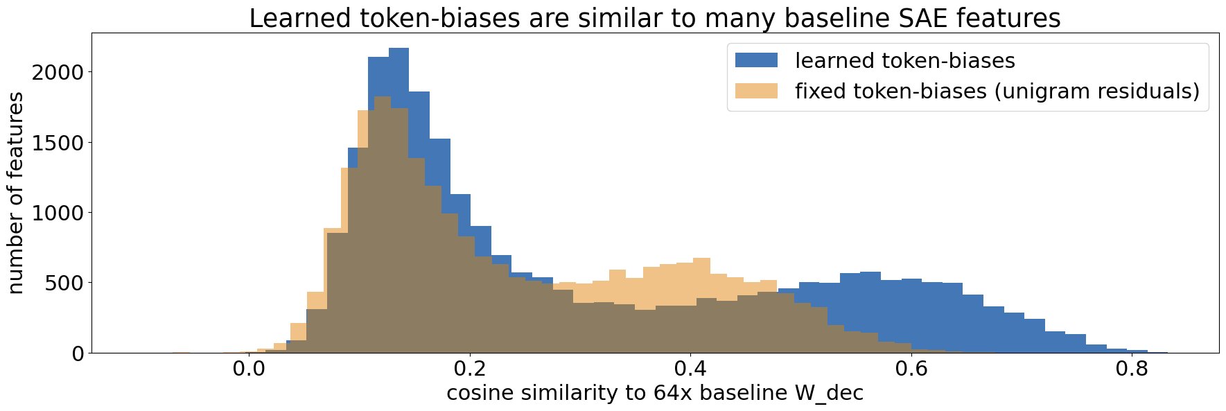
That said, ~25% of the suggested 64x baseline features are similar to the token-biases (cosine similarity 0.4-0.9). In fact, evolving the token-biases via training substantially increases their similarity (see figure). Smaller expansion sizes have up to 66% similar features and fewer dead features. (related sections above: 'Dead features' and 'Measuring "simple" features')
Do you have a dictionary-size to CE-added plot? (fixing L0)
So, we did not use the lookup biases as additional features (only for decoder reconstruction)
I agree it's not like the other features in that the encoder isn't used, but it is used for reconstruction which affects CE. It'd be good to show the pareto improvement of CE/L0 is not caused by just having an additional vocab_size number of features (although that might mean having to use auxk to have a similar number of alive features).
One caveat that I want to highlight is that there was a bug training the tokenized SAEs for the expansions sweep, the lookup table isn't learned but remained at the hard-coded values...
They are therefore quite suboptimal. Due to some compute constraints, I haven't re-run that experiment (the x64 SAEs take quite a while to train).
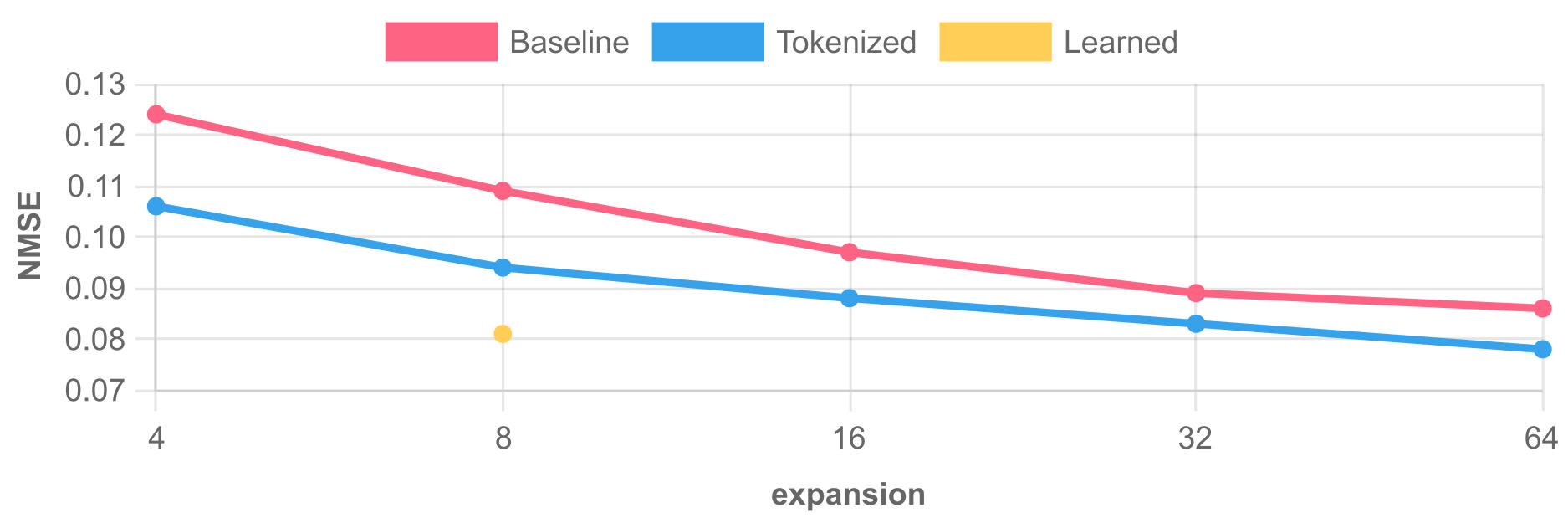
Anyway, I think the main question you want answered is if the 8x tokenized SAE beats the 64x normal SAE, which it does. The 64x SAE is improving slightly quicker near the end of training, I only used 130M tokens.
Below is an NMSE plot for k=30 across expansion factors (the CE is about the same albeit slightly less impacted by size increase). the "tokenized" label indicates the non-learned lookup and the "Learned" is the working tokenized setup.
That's great thanks!
My suggested experiment to really get at this question (which if I were in your shoes, I wouldn't want to run cause you've already done quite a bit of work on this project!, lol):
Compare
1. Baseline 80x expansion (56k features) at k=30
2. Tokenized-learned 8x expansion (50k vocab + 6k features) at k=29 (since the token adds 1 extra feature)
for 300M tokens (I usually don't see improvements past this amount) showing NMSE and CE.
If tokenized-SAEs are still better in this experiment, then that's a pretty solid argument to use these!
If they're equivalent, then tokenized-SAEs are still way faster to train in this lower expansion range, while having 50k "features" already interpreted.
If tokenized-SAEs are worse, then these tokenized features aren't a good prior to use. Although both sets of features are learned, the difference would be the tokenized always has the same feature per token (duh), and baseline SAEs allow whatever combination of features (e.g. features shared across different tokens).
This is a completely fair suggestion. I'll look into training a fully-fledged SAE with the same number of features for the full training duration.
Although, tokenized features are dissimilar to normal features in that they don't vary in activation strength. Tokenized features are either 0 or 1 (or norm of the vector). So it's not exactly an apples-to-apples comparison w/ a similar sized dictionary of normal SAE features, although that plot would be nice!
Did you ever do a max-cos-sim between the vectors in the token-biases? I'm wondering how many biases are exactly the same (e.g. " The" vs "The" vs "the" vs " the", etc) which would allow a shrinkage of the number of features (although your point is good that an extra vocab_size num of features isn't large in the scale of millions of features).
Indeed, similar tokens (e.g. "The" vs. " The") have similar token-biases (median max-cos-sim 0.89). This is likely because we initialize the biases with the unigram residuals, which mostly retain the same "nearby tokens" as the original embeddings.
Due to this, most token-biases have high cosine similarity to their respective unigram residuals (median 0.91). This indicates that if we use the token-biases as additional features, we can interpret the activations relative to the unigram residuals (as a somewhat un-normalized similarity, due to the dot product).
That said, the token-biases have uniquely interesting properties -- for one, they seem to be great "last token detectors". Suppose we take a last-row residual vector from an arbitrary 128-token prompt. Then, a max-cos-sim over the 50257 token-biases yields the prompt's exact last token with 88-98% accuracy (layers 10 down to 5), compared to only 35-77% accuracy using unigram residuals (see footnote 2).
Do you have any tokenized SAEs uploaded (and a simple download script?). I could only find model definitions in the repos.
If you just have it saved locally, here's my usual script for uploading to huggingface (just need your key).
We used a google drive repo where we stored most of the runs (https://drive.google.com/drive/folders/1ERSkdA_yxr7ky6AItzyst-tCtfUPy66j?usp=sharing). We use a somewhat weird naming scheme, if there is a "t" in the postfix of the name, it is tokenized. Some may be old and may not fully work, if you run into any issues, feel free to reach out.
The code in the research repo (specifically https://github.com/tdooms/tokenized-sae/blob/main/base.py#L119) should work to load them in.
Please keep in mind that these are currently more of a proof of concept and are likely undertrained. We were hoping to determine the level of interest in this technique before training a proper suite.
Additionally:
- We recommend using the
gpt2-layersdirectory, which includes resid_pre layers 5-11, topk=30, 12288 features (the tokenized "t" ones have learned lookup tables, pre-initialized with unigram residuals). - The folders
pareto-sweep,init-sweep, andexpansion-sweepcontain parameter sweeps, with lookup tables fixed to 2x unigram residuals.
In addition to the code repo linked above, for now here is some quick code that loads the SAE, exposes the lookup table, and computes activations only:
import torch

SAE_BASE_PATH = 'gpt2-layers/gpt2_resid_pre'                   # hook_pt = 'resid_pre'

layer = 8
state_dict = torch.load(f'{SAE_BASE_PATH}_{layer}_ot30.pt')    # o=topk, t=tokenized, k=30
W_lookup = state_dict['lookup.W_lookup.weight']                # per-token decoder biases

def tokenized_activations(state_dict, x):
    'Return pre-relu activations. For simplicity, does not limit to topk.'
    return (x - state_dict['b_dec']) @ state_dict['W_enc'].T + state_dict['b_enc']
This work is really interesting. It makes sense that if you already have a class of likely features with known triggers, such as the unigrams, having a lookup table or embeddings for them will save in compute, since you don't need to learn the encoder.
I wonder if this approach could be extended beyond tokens. For example, if we have residual stream features from an upstream SAE does it make sense to use those features for the lookup table in a downstream SAE. The vectors in the table might be the downstream representation of the same feature (with updates from the intermediate layers). Using features from an early layer SAE might capture the effective tokens that form by combining common bigrams and trigrams.
Tokens are indeed only a specific instantiation of hardcoding "known" features into an SAE, there are lots of interesting sparse features one can consider which may even further speed up training.
I like the suggestion of trying to find the "enriched" token representations. While our work shows that such representations are likely bigrams and trigrams, using an extremely sparse SAE to reveal those could also work (say at layer 1 or 2). While this approach still has the drawback of having an encoder, this encoder can be shared across SAEs, which is still a large decrease in complexity. Also, the encoder will probably be simpler since it's earlier in the model.
This idea can be implemented recursively across a suite of SAEs, where each layer can add to a pool of hardcoded features. In other words, each layer SAE in a layer has its own encoder/decoder and the decoder is copied (and fine-tuned) across later layers. This would allow to more faithfully trace a feature through the model than is currently possible.
tl;dr
The proposed lookup table 'hardcodes' these token subspaces and reduces the need to learn these local features, which results in more interesting/complex learned features. We perform a blind feature evaluation study and quantitative analysis showing that unigram-based ("simple") features are much less frequent.
For some interesting results about token subspaces, see our Motivation. To skip to feature quality, see Feature Evaluation. For those interested in training SAEs, skip to Technical Discussion.
We also publish the research code and simplified code of Tokenized SAEs and a dataset of the most common n-grams in OpenWebText (used in Motivation).
Introduction
Sparse auto-encoders (SAEs) are a promising interpretability method that has become a large focus of the mechinterp field. We propose augmenting them with a token-based lookup table, resulting in rapid, high-quality training. Specifically,
Motivation: Residuals ~ Unigram Residuals
To rationalize adding a per-token vector, we will experimentally show that:
n-grams Strongly Approximate Residual Activations
To predict the next word in a sentence, the preceding few words often are most important. Similarly, an LLM's residual activations have strong cosine similarity to that of their last n-gram. In other words, we compare activations of an input sequence [BOS, <tok1>, ..., <tokN>] to that of solely its last-token unigram [BOS, <tokN>][1].
Regardless of model complexity and layer depth, we find a consistently strong cosine similarity between these (in fact, the last token is very often the most similar[2]):
This similarity increases with n as more context becomes available. For example, in gpt2-small we find that trigrams often provide a good approximation of the full residuals:
Therefore, residual activations are often very similar to those of their last few tokens. We hypothesize this is a large factor why SAE features often activate on and reconstruct particular tokens or token sequences.
A Training Imbalance Biases SAEs Toward Local Context
Sparse auto-encoders may be additionally biased toward local context due to a strong training class imbalance[3]. During training, short n-grams are exponentially over-represented, leading the SAE to memorize them more precisely.
The precise imbalance is proportional to the training set token frequency[4]. By counting how often particular n-grams occur in OpenWebText, we see that about 2000 n-gram representations are presented to the SAE in a potential ratio of >1M to one:
In a typical classifier such as logistic regression, a major training class imbalance leads to the model memorizing the most prevalent class via model biases. We find this also occurs in SAEs, which is essentially a set of logistic regressors trained in tandem.
In SAEs, each common token results in a well-defined subset of features to strongly activate. These subsets are clearly visible by presenting common n-gram residual activations to the SAE:
This results in the SAE hidden layer effectively modeling the most common n-grams:
This implies that observing which unigrams (or common bigrams/trigrams/etc) activate a given feature is often predictive of which tokens the feature will activate on in longer prompts.[5]
This also implies that the latent reconstruction MSE is inversely correlated with training set token frequency:
A similar correlation also exists for common bigrams but is not as prominent. We hypothesize this is because the most common bigrams are composed of the most common unigrams, hence they are already in the subspace of the last token:
We found that in later layers, more SAE features activate to common bigrams than unigrams. In fact, many later-layer features do not respond to any short n-gram (e.g. ~24% in RES-JB layer 8). This is potentially because the most common activations at that point are no longer unigram-like, but are a result of non-local information averaged by attention.
The Tokenized SAE: Adding a Lookup Table
SAEs are trained to reconstruct latent representations, applying L1 regularization to encourage sparsity. The resulting SAE hidden layer ("feature") activations are observed to correlate with interesting patterns in the prompt.
We have experimentally demonstrated the importance of the last-token subspace, both to the model and SAEs. Because we can estimate this direction in advance, we can add it to the SAE decoder, stored in a lookup table Wlookup. In practice, we initialize the lookup table with unigram activations and allow the training procedure to learn them from there.
We hypothesize this will improve training speed and remove "simple" (unigram-based) features. Conceptually, Tokenized SAEs are straightforward; they are identical to an ordinary SAE, except for this token-specific lookup table. This amounts to the following in a standard SAE:
f(x)=σ(Wenc(x−bdec))
^x=Wdec(f(x))+bdec+Wlookup(t)
Here, x represents the input activations at a certain point in the model for a certain token t. Wlookup is a matrix where each row corresponds to the bias for a specific token. Implementing this addition in the forward code of the SAE itself is trivial (i.e. incorporating the term only with the decoder).
Just for emphasis, this technique can be applied to any architecture. In the final SAE, no change is necessary to the encoder math. The lookup table is only required if it is desired to reconstruct the activations.
Tokenized SAE Evaluation
We will now quantitatively and qualitatively examine the results of adding the decoder lookup.
Quantitative Results
Reconstruction
We start with the ubiquitous Pareto plot for all tested SAEs on GPT-2 layer 8. We trained on more than 300M tokens to the point all metrics no longer meaningfully decreased. We measure the NMSE (MSE divided by the L2 norm of the target) and CE added (% of increased CE loss).
Next, we show the CE loss across layers on GPT-2 small, using a TopK SAE as the baseline. These SAEs all use k=30. The MSE follows a similar pattern.
The TSAE is better by a fair margin across all layers. This also shows that the TSAE reconstruction does not deteriorate with depth (relative to the baseline), as one would expect. In the Motivation section, we showed evidence that in larger models and later layers, residuals are still very similar to unigram residuals. Toward this, we generated TopK TSAEs for Pythia 1.4B layers 12, 16, and 20. Despite being undertrained (70M tokens), the training progression shows no signs of the baseline "catching up". Here are the CE added for k=50 (the NMSE exhibits similar improvement):
Again, TSAEs achieve considerably lower reconstruction and CE. We did not micro-optimize any hyperparameters, choosing one consistent value across all experiments.
Training Dynamics
Beyond tokenized SAEs beating their baselines in most regards, we specifically wish to highlight their training speed. The following plot shows the speedup gain, measured by taking the final value of a given metric for TopK SAEs and then looking at which point TSAEs crossed that threshold. We then show that fraction.
This speedup is huge across the board (and even increases by depth). This brings training times for competitive reconstruction down to mere minutes. We believe this to be the main advantage of tokenized SAEs; they provide a way to train full suites of SAEs within the hour, which can be handy for circuit analysis.
Overhead
Computationally, we found tokenized SAEs to have a 5% overhead (excluding gathering activations) on a GTX 4080 compared to an ordinary TopK SAE. We expect this could be mostly optimized away through some low-level implementation tricks.
In terms of memory, the lookup table is a large constant factor that tends to dominate small SAEs. Our SAEs on GPT-2 use an expansion factor of 16; the lookup table triples the total size. We wish to stress that SAE size is generally not a constraining factor, loading our SAEs for each layer of the residual amounts to 3GB of memory. However, if this is an issue one can probably get away by only considering a lookup table for a subset of common tokens. We haven't yet looked into what the impact is of such a change but expect it's possible to get away with only using the top half of the most common tokens.
Dead features
One current deficiency of TSAEs is that they generally have more dead features. This ranges from twice as many dead features as TopK to the amount being almost the same. The layer 5-10 gpt2-small TSAEs resulted in 10%-50% dead features, decreasing with layer.
We haven't yet determined the cause (beyond the obvious) or tried any techniques to resolve this. A promising approach would be to use the auxK described here. If this were solved, we believe both training times and final loss to decrease.
Because we pre-initialize each feature with the encoder and decoder weights transposed, an interesting finding is that dead features correspond nearly exactly to features with high cosine similarity between each feature's encoder and decoder. This can be used post-facto to detect dead features:
We examined the high-similarity group using four metrics, concluding they are likely not valid features:
Measuring "simple" features
First, we define "simple" features as unigram-based. To measure whether features detect these (or represent them), we can determine the cosine similarity between the feature encoder/decoder weights and unigram activations. In doing this, we discover that the tokenized version of TopK SAE substantially lacks unigram representations in comparison in GPT2-small layer 8:
The cosine similarity of the encoder weights is lower since the decoder tends to represent directions existing in the activations while the encoder performs a somewhat fuzzy match. This leads to a mean cosine similarity of ~0.2-0.4, which may be lower than assumed. However, keep in mind each feature likely must handle quite a bit of noise and therefore doesn't want to match too strongly.
In terms of the decoder, in GPT-2 the cosine similarity between two closely related tokens (eg "cat" and "Cat") is generally between 0.5 and 0.8. We find that most unigram features learn these features at once, leading to a similarity of ~0.4 on average.
A second way to measure "simple" features is by measuring how many features still strongly activate[6] with only the last n tokens. If the feature still strongly activates with the last two tokens, for example, this perhaps implies the feature may not represent the earlier context.
Therefore, we measure the minimum n that causes (a) a positive activation (indicating perhaps the start of an increasing sequence), and (b) is within 90% of the maximum activation (indicating a strong encoder weight similarity of the input). [7]
The results re-affirm that unigram features are less prevalent in tokenized, and they show that TSAEs nearly always have a larger percentage of complex features at every n > 2:
Qualitative Results
Feature Quality
We measure the perceived quality of features in comparison to our baseline SAEs and RES-JB according to Cunningham & Connerly (2024) [8]. We manually score 20 features from standard and TopK SAEs, with tokenized variants denoted with an asterisk. We rank complexity from 1 (unigrams) to 5 (deep semantics), and consistency from 1 (no discernable pattern) to 5 (no deviations). Note these results should be interpreted cautiously due to the limited sample size:
To illustrate this further, we provide a subjective categorization of the first 25 features of the TopK Tokenized SAE. Our purpose is not to over-generalize, but to demonstrate that TSAE features seemingly have complexity:
To show the feature breadth, we have included additional interesting features in the footnotes[6].
Feature Complexity Measures
We hypothesize that tokenized SAEs reduce the number of "simple" features which activate primarily on the final token. We approximate this using the following method [7].
First, we measure how many tokens are directly activated by features. If a feature is only activated by a few tokens, its decoder is more likely to reconstruct that token exactly (making it somewhat of a "feature reconstruction token", which we describe as a "simple" feature).
We see that individual tokens are rarely represented in small tokenized SAEs, while "simple" features are perhaps overly prevalent in large ones:
Technical Details
Now, we will share some details for effectively training tokenized SAEs. This section may be more technical than others.
Caching Tokens
SAEs have three modi operandi: training, activating, and reconstructing. We'll now examine how the lookup table affects each.
Generally, SAEs are trained by sampling (collecting) activations into a big buffer and shuffling those (to remove the context dependence which may lead to micro-overfitting and consequently unstable training).
Initializing the Lookup Table
SAE encoders are often initialized to the transpose of their decoder, aiming to approximate an identity operation. Anecdotally, this has a large positive impact on convergence speed but also the converged reconstructions.
Similarly, we found that a properly initialized lookup table significantly helps training better SAEs. To achieve this we use unigram reconstructions (explained above). They provide a good baseline for the SAE features to build upon.
One can imagine taking other approaches, such as taking the mean of activations for each token over a certain dataset. We haven't performed a rigorous ablation to test this. Our intuition of using unigram reconstruction (including attention sink) over the alternatives is that there is less noise that may be somehow pathological or otherwise biased. In that sense, we are choosing the "purest" token reconstruction baseline.
Furthermore, instead of using the exact initialization described above, we've found that it's important to "balance" the lookup table and the SAE itself. We do this by settingWenc=(1−α)WTdec and Wlookup=αWunigram. This α can be interpreted as "how much token subspace we predict there to be". Clearly, an optimal value will depend on model and depth but we've found that, somewhat surprisingly, a value of 0.5 is almost universally optimal (or at least a very good guess) [10].
During training, we measure the evolution of this balance via the lookup table. We measure the following (scale-aware) cosine similarity:
^α=Wlookup⋅Wunigram||Wunigram||2
For SAEs on the residual stream of GPT-2, this ^a varies from 0.6 (layer 5) to 0.5 (layer 11). In Pythia 1.4b we did not do a full ablation but it settled at 0.43 on layer 16.
There is no guarantee that ^α will reach the "optimal" value for any start α . For instance if α=0 , then ^α may converge towards 0.3. However, if we start another run with α=0.3, then ^α rises towards 0.5 (with better loss metrics). This indicates that the SAE struggles to find good optima on itself for the lookup table.
Learning the Lookup Table
One potential pitfall in implementing TSAEs is that the learning rate of the lookup table should be higher than the SAE itself. At first, it may not seem obvious why given we use lookup tables all the time. The difference is that we're summing them, not chaining them.
When using TopK SAEs, it's more easily understood. Since k features are active at a time, on average, each SAE feature will be updated k times more than the lookup table features. Empirically, we found that setting the lookup learning rate higher (more than scaled by k) yields better results. We believe this to be due to a combination of the token bias being more stable, dead features (resulting in some features being updated much more) and varying token frequencies.
PyTorch's embedding class also allows dynamic learning rates according to entry frequency (tokens in our case). We didn't try this, but it may further improve learning a correct lookup table.
Discussion
While TSAEs may not seem like a big change, they require a slight adaptation in how we think about SAEs. In this section, we cover TSAEs from two angles: discussing some possible criticisms of this approach, then outlining some more optimistic outlooks.
Devil's Advocate
There are some weaknesses to the proposed approach. We believe the main points boil down to the following.
While we believe all arguments have merit, we claim they are generally not as strong as one might think. The following are one-line counterarguments to each of them.
Token Subspace Importance
Our experiments show that context-aware embeddings bear considerable similarity to simple unigram embeddings, even in deeper models. This leads us to believe that the token subspace is universally the most important subspace towards reconstructing embeddings. While longer contexts and deeper models may dilute this subspace, we expect this to be generally true.
Wider SAEs
As stated before, the community generally doesn't have the computing power or storage capacity to train and use multi-million-feature SAEs. Even if SAEs remain the prominent direction in mechinterp, we do not believe this fact to change soon.
On a different note, the recent TopK Paper describes feature clustering results (Appendix 7), which indicate that large SAEs generally organize themselves into two main categories. They also note that this smaller cluster (about 25%) fires more strongly for select tokens while the other cluster fires more broadly. This is very closely related to what our analysis showed and what was the main motivation for TSAEs. We cautiously hypothesize that TSAEs may scale beyond our current results (potentially with some tweaks).
Inductive bias = bad
There are several ways that this concern can be formulated. It generally boils down to noting that a token-based lookup table constrains the SAE in a way that may be unhelpful or even counterproductive. It's generally hard to completely refute this argument since we can't check all possible scenarios. TSAEs can fail in two ways: bad metrics and bad feature quality.
Broadly speaking, inductive bias has played a large role in ML. Just as residuals assume that most computation is shallow and should be somewhat enforced, we assume certain features to be prominent. Along the same lines, inductive biases can play a role in interpretability research to simplify and constrain certain analysis methods.
Angel's Advocate
From experience, some important upsides are not immediately clear upon first hearing about TSAEs. This is a subjective list of less obvious advantages to our approach.
Lookup Table for Interpretability
TSAEs are incentivized to push anything token-related to the lookup table and anything context-related to the SAE. This results in a natural disentanglement of these concepts. Since the trigger is deterministic, there is no need to figure out what activates a feature. We simply get a bunch of clear and meaningful directions in latent space. This can be seen as an intermediate embedding table that may be more meaningful than the original embedding for circuit analysis.
Less confusing feature splitting
Feature splitting seems like a fact of life for SAEs, they can make features less interpretable and less useful for steering. TSAEs have the advantage that the pure dictionary features are much less likely to devolve to a concept but for specific tokens feature (eg. "the" in math context). The most common form of feature splitting will be more specific contexts/concepts, which we believe to be less harmful. We have not yet done a study into this claim.
Similar Work
The present work can be applied to any SAE architecture. Some recent sparse auto-encoder methods build specifically on TopK SAEs (Gao et al.):
Other techniques can be used more generally. For example, researchers have explored alternative activation functions (e.g. JumpReLU, Rajamanoharan et al.) and loss functions (e.g. p-annealing, Karvonen et al.).
Conclusion
We showed that tokenized SAEs produce interesting features in a fraction of the training time of standard SAEs. We provided evidence the technique is likely to scale to larger models and trained some Pythia 1.4B TSAEs, which seemingly have good features. There are also additional avenues for future research. For example, potentially incorporating lookups for larger n-grams and more thoroughly investigating feature quality.
Lastly, we hope this study will ignite further research towards not simply scaling SAEs but making them more structured in interpretable ways.
By default, we retain the BOS token for the simple reason that it has been found to be important in the role of attention sinking. Removing the BOS has been shown to break model performance in strange ways.
Across ~38K 128-token prompts, we can measure the percentage when the last token unigram is most similar to the residuals, of all other unigrams. Surprisingly, this occurs >20% of the time across all layers and models tested. Here, Gemma 2B has ~256K tokens, while the others have ~52K. Also, we consider "nearby/near-exact" tokens to be when their string representation is identical following token.strip().lower() (in Python).
We use the terminology "imbalance" because it accurately describes the expected effect -- bias toward particular over-represented classes. However, technically speaking this is best described as a "weighted regression class".
Every input sequence [BOS, <tok1>, <tok2>, ...] results in training the SAE to reconstruct the representations of [BOS], [BOS, <tok1>], [BOS, <tok1>, <tok2>], etc. So, the SAE will see the [BOS] representation for every training example, while n-gram representations will follow the distribution of the n tokens in the training set.
In RES-JB layer 8, we found that 76% of features are activated by a unigram. Of these, 39% matched the top unigram activation and 66% matched at least one.
To show additional breadth, we have included some more features:
• 36: ”.\n[NUM].[NUM]”
• 40: Colon in the hour/minute ”[1-12]:”
• 1200: ends in ”([1-2 letters])”
• 1662: ”out of [NUM]”/”[NUM] by [NUM]”/”[NUM] of [NUM]”/”Rated [NUM]”/”[NUM] in [NUM]”
• 1635: credit/banks (bigrams/trigrams)
• 2167: ”Series/Class/Size/Stage/District/Year” [number/roman numerals/numeric text]
• 2308: punctuation/common tokens immediately following other punctuation
• 3527: [currency][number][optional comma][optional number].
• 3673: ” board”/” Board”/” Commission”/” Council”
• 5088: full names of famous people, particularly politicians
• 5552: ends in ”[proper noun(s)]([uppercase 1-2 letters][uppercase 1-2 letters]”
• 6085: ends in ”([NUM])”
• 6913: Comma inside parentheses
It is important to note that current complexity methods are likely inexact. Feature activations may be caused by conjunctive factors which obscure their true basis, e.g. specific final tokens, sequence position, and repeated tokens/patterns from earlier in the prompt. For example, a feature that does not respond to unigrams (or overly responds to them) may simply have a strong positional bias. Separating these factors is complex and not a subject of this paper.
Cunningham, H. and Connerly, T. Circuits updates - June 2024. Transformer Circuits Thread, 2024.
SAE feature activations were stongly correlated with cosine similarity between the input vector and encoder weights. This follows directly from the encoder computation. A small feature activation implies a low cosine similarity, risking that the feature was activated by chance. It therefore seems advisable to set a minimum activation threshold for qualitative work. For a layer 8 TopK tokenized SAE:
It generally doesn't matter if we scale either the encoder or decoder. This was just slightly simpler to notate. Note that some SAE variants force their decoder row norm to be 1, which would negate this initialization.
Experiments are based on gpt2-small layer 8. It is sufficiently deep in the model that we would expect complex behavior to have arisen.
The formulas are as follows:
CEadded(x)=(CEpatched(x)−CEclean(x))CEclean(x)
NMSE(x)=||x−SAE(x)||2||x||2