- Global Threshold - Let's treat all features the same. Set all feature activations less than [0.1] to 0 (this is equivalent to adding a constant to the encoder bias).
The bolded part seems false? This maps 0.2 original act -> 0.2 new act while adding 0.1 to the encoder bias maps 0.2 original act -> 0.1 new act. Ie, changing the encoder bias changes the value of all activations, while thresholding only affects small ones
Why is CE loss >= 5.0 everywhere? Looking briefly at GELU-1L over 128 positions (a short sequence length!) I see our models get 4.3 CE loss. 5.0 seems really high?
Ah, I see your section on this, but I doubt that bad data explains all of this. Are you using a very small sequence length, or an odd dataset?

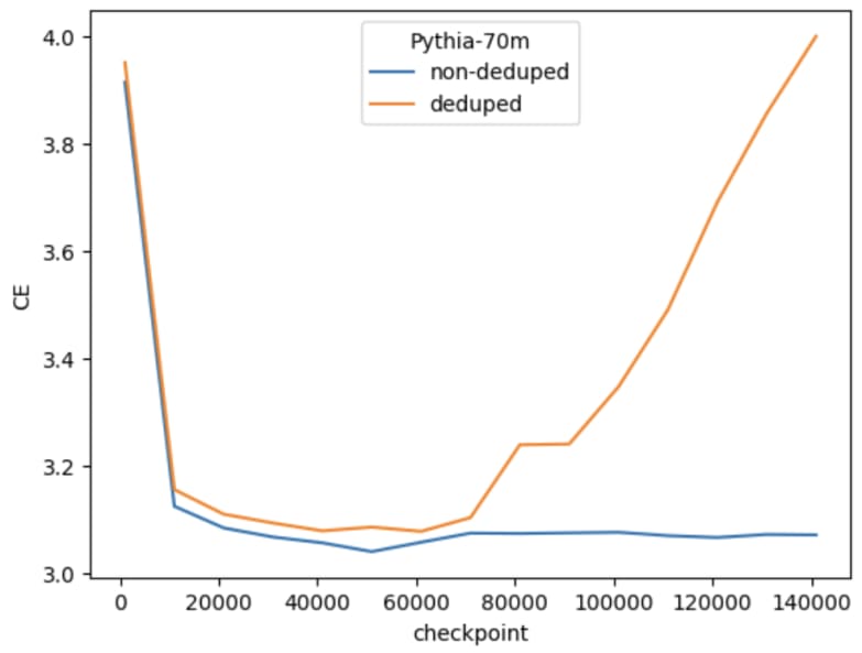
There actually is a problem with Pythia-70M-deduped on data that doesn't start at the initial position. This is the non-deduped vs deduped over training (Note: they're similar CE if you do evaluate on text that starts on the first position of the document).
We get similar performing SAE's when training on non-deduped (ie the cos-sim & l2-ratio are similar, though of course the CE will be different if the baseline model is different).
However, I do think the SAE's were trained on the Pile & I evaluated on OWT, which would lead to some CE-difference as well. Let me check.
Edit: Also the seq length is 256.
Yep, there are similar results when evaluating on the Pile with lower CE (except at the low L0-end)

Thanks for pointing this out! I'll swap the graphs out w/ their Pile-evaluated ones when it runs [Updated: all images are updated except the one comparing the 4 different "lowest features" values]
We could also train SAE's on Pythia-70M (non-deduped), but that would take a couple days to run & re-evaluate.
TL;DR
We achieve better SAE performance by:
with 'better' meaning: we can reconstruct the original LLM activations w/ lower MSE & with fewer features/datapoint.
As a sneak peak (the graph should make more sense as we build up to it, don't worry!):
Now in more details:
Sparse Autoencoders (SAEs) reconstruct each datapoint in [layer 3's residual stream activations of Pythia-70M-deduped] using a certain amount of features (this is the L0-norm of the hidden activation in the SAE). Typically the higher activations are interpretable & the lowest of activations non-interpretable.
Here is a feature that activates mostly on apostrophe (removing it also makes it worse at predicting "s"). The lower activations are conceptually similar, but then we have a huge amount of tokens that are something else.
From a datapoint viewpoint, there's a similar story: given a specific datapoint, the top activation features make a lot of sense, but the lowest ones don't (ie if 20 features activate that reconstruct a specific datapoint, the top ~5 features make a decent amount of sense & the lower 15 make less and less sense)
Are these low-activating features actually important for downstream performance (eg CE)? Or are they modeling noise in the underlying LLM (which is why we see conceptually similar datapoints in lower activation points)?
Ablating Lowest Features
There are a few different ways to remove the "lowest" feature activations.
Dataset View:
Feature View: Features have different activation values. Some are an OOM larger than others on average, so we can set feature specific thresholds.
It turns out that the simple global threshold performs the best:
[Note: "CE" refers to the CE when you replace [layer 3 residual stream]'s activations with the reconstruction from the SAE. Ultimately we want the original model's CE with the smallest amount of feature's per datapoint (L0 norm).]
You can halve the L0 w/ a small (~0.08) increase in CE. Sadly, there is an increase in both MSE & CE. If MSE was higher & CE stayed the same, then that supports the hypothesis that the SAE is modeling noise at lower activations (ie noise that's important for MSE/reconstruction but not for CE/downstream performance). But these lower activations are important for both MSE & CE similarly.
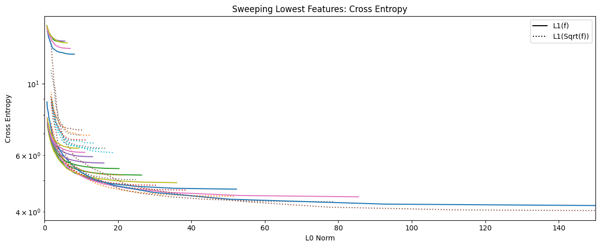
For completion sake, here's a messy graph w/ all 4 methods:
[Note: this was run on a different SAE than the other images]
There may be a more sophisticated methods that take into account feature-information (such as whether it's an outlier feature or feature frequency), but we'll be sticking w/ the global threshold for the rest of the post.
Sweeping Across SAE's with Different L0's
You can get widly different L0's by just sweeping the weight on the L1 penalty term where increasing the L0 increases reconstruction but at the cost of more, potentially polysemantic, features per datapoint. Does the above phenomona extend to SAE's w/ different L0's?
Looks like it does & the models seems to follow a pareto frontier.
Using L1(sqrt(feature_activation))
@Lucia Quirke trained SAE's with L1(sqrt(feature_activations)) (this punishes smaller activations more & larger activations less) and anecdotally noticed less of these smaller, unintepretable features. Maybe this method can get us better L0 for the same CE?
In fact it does! Whoooo! Though, becomes pareto worse at around SAE's with ~15 L0 norm.
But in what way is this helping? We can break the loss into a couple components:
1. Cos sim: when reconstructing an activation, how well does the SAE approximate the direction? ie a cos-sim of 1 means the reconstruction is pointing in the same direction, but might not be the same magnitude
2. L2 Ratio: How well does the SAE reconstruct the magnitude of the original activation?
Most strikingly, it helps with the L2 Ratio significantly:
This makes sense because higher activating feature activations are punished less for the sqrt() than otherwise. If you have higher-activating features, they can reconstruct the norm better even with the decoder normalization constraint. Looking at Cos sim & MSE we see similar improvements.
What about L1(sqrt(sqrt()))?
If sqrt-ing helped, why not do more?
It got worse than just one sqrt, lol.
Looking at the graph of these loss terms:
Sqrt-ing does decrease low (<1.0) feature-activations more & higher (>1.0) feature-activations less relative to the usual L1 penalty. The point of 1 & the slope of sqrt are arbitrary with respect to the feature activations (ie other points/slopes may perform better)
For example, look at a few datapoint activations:
We do see a right shift in activations for L1(sqrt()) as expected. But the median activation is 0.28 & 0.43 for L1 & L1(sqrt()) respectively. Lets say we want to punish values around 0.01 more, but once it becomes 0.1, we don't want to punish as much. We could then do sqrt(0.1*x).
We could also sweep this [0.1] value as a parameter (while trying to maintain a similar L0 which is tricky) as well as trying slopes between x & x^0.25 (ie sqrt(sqrt())).
Feature Frequency/Density Plots
Anthropic noticed that very low frequency feature activations were usually uninterpretable (note: they say low "density" where I say low "frequency").
We do see more low-frequency features for L1(sqrt()) here.
[Note: I chose 1e-5 as the threshold based off the feature frequency histograms in the appendix]
Future Work
It'd be good to investigate a better L1 penalty than L1(sqrt(x)). This can be done empirically by throwing lots of L1 loss terms at the wall, or there may be a more analytical solution. Let me know if you have any ideas! Comments and dms are welcome.
We also give intermediate results & discussion in the EleutherAI Sparse-coding channel; feel welcomed to join the discussion!
Invite to the server and link to our project thread
Appendix
Feature Freq histograms