This work was done as part of MATS 7.0. We consider this in-progress research and we are grateful for any thoughts and feedback from the community.
Update (May 20, 2025): This is now a paper! Check out our paper "Feature Hedging: Correlated Features Break Narrow Sparse Autoencoders" (arxiv.org/abs/2505.11756).
Update (April 4, 2025): We found that hedging caused by positive (but not hierarchical) correlation between features can sometimes be removed with a high enough sparsity penalty, but this is never true for hedging caused by hierarchical features or negatively correlated features. We have updated the post accordingly.
Introduction
If there is any correlation between a feature captured by an SAE and a feature not captured by that SAE, the SAE will merge the external feature into its latent tracking the internal feature. This phenomenon, which we call feature hedging, is caused by MSE reconstruction loss and will happen any time the SAE is both too narrow to capture all the “true features” in the model, and there is correlation between the features tracked by the SAE and the features not tracked by the SAE. Both of these conditions are almost certainly true of every SAE trained on an LLM, especially narrower SAEs like the inner parts of Matryoshka SAEs. This means all LLM SAE latents likely have spurious components of correlated features mixed in, harming the performance of the SAE and likely contributing to the underwhelmingperformance of SAEs.
We also present a novel reconstruction loss, called snap loss, which solves feature hedging in toy models. However, it does not work if the amount of feature correlation is too high, or there are too many correlated features; so snap loss may not be useful in real LLM SAEs.
When an SAE is too narrow to represent two correlated features, MSE loss incentivizes the SAE to mix components of both features into its latent to reduce a large squared-error penalty when the secondary feature fires. This causes the SAE to learn incorrect latents that mix components of multiple features together.
In this post, we begin by defining feature hedging and comparing it to feature absorption. We then demonstrate hedging using a simple toy model of a single-latent SAE. We present snap loss as a potential solution to hedging that works in toy models, but it is not clear if it improves LLM SAEs. We then explore hedging in Matryoshka SAEs with and without snap loss. We finish by presenting evidence that hedging is occurring in LLM SAEs, and conclude with some results we are uncertain about.
While both feature absorption and feature hedging can be consequences of co-occurring features, the underlying causes and effects of each are very different. The table below summarizes the differences between hedging and absorption.
Feature absorption
Feature hedging
Learns gerrymandered latents
Mixes correlated features into latents
Caused by sparsity
Caused by MSE loss
Relevant features are tracked in the SAE
One feature is in the SAE, the other is not
Asymmetry between encoder and decoder
Affects encoder and decoder symmetrically
Gets worse the wider the SAE
Gets worse the narrower the SAE
Requires hierarchical features
Requires only correlation between features
Background: feature absorption
In featureabsorption, there is a parent feature fp and a child feature fc in a hierarchical relationship. If fc is active then fp must also be active, so that fc⟹fp. In order to increase sparsity, an SAE that is wide enough to track both fc and fp in their own latents will, unfortunately, not learn latents l0=fp and l1=fc. Instead, the SAE can increase sparsity by merging fc and fp together in the decoder of l1, and encode ¬fc∧fp in the encoder of l0. Thus, l0 appears to track fp but does not fire when both fp and fc are active, and l1 appears to track fc but actually contains both fc and fp in its decoder. This is demonstrated below.
The encoder and decoder vs true feature cosine similarity for a sample 2-latent SAE exhibiting feature absorption is demonstrated below.
Cosine similarity of SAE latents vs true features exhibiting feature absorption. Latent 0 appears to track the parent feature (feature 0), but its encoder turns the latent off when the child feature (feature 1) is active. Latent 1 appears to track the child feature (feature 1), but its decoder mixes both features together. This asymmetry between the encoder and decoder is characteristic of feature absorption.
Comparing feature hedging and feature absorption
In feature hedging, there is a main feature fm that is tracked in a narrow SAE by latent l0. There is a secondary feature fs whose firing is positively or negatively correlated with fm, but the SAE is too narrow to assign a latent to track fs. If fs is positively correlated with fm, then the SAE will learn l0=fm+αfs in both the encoder and decoder, where 0<α<1. If fs is negatively correlated with fm, then the SAE learns fm−αfs. In both cases, the SAE latent l0 learns a mixture of fm and fs as this minimizes MSE loss relative to the ideal solution we would like the SAE to learn, which is simply l0=fm.
A special case of this is where fs⟹fm, which is the hierarchical relationship from feature absorption where fs=fc and fm=fp, as hierarchy is simply a very strong form of correlation between features. We show an equivalent example for what hedging looks like using the feature absorption example from above but in a SAE too narrow to represent both:
The encoder and decoder vs true feature cosine similarity for a sample single-latent SAE exhibiting feature hedging with hierarchical features is demonstrated below. These same features would result in feature absorption if the SAE was wide enough to represent both features.
Cosine similarity of SAE latents vs true features exhibiting feature hedging. The SAE is too narrow to represent both the main feature (feature 0) and the secondary feature (feature 1). Since these features are correlated, a small component of feature 1 is mixed into feature 0 in both the encoder and decoder. Feature hedging affects the encoder and decoder roughly symmetrically.
Feature absorption is a problem caused by the sparsity penalty in wide SAEs, which implies that using narrow SAEs like in Matryoshka SAEs could be a solution. However, hedging shows that reconstruction loss can also cause issues, and is especially bad the more narrow the SAE, making solving both hedging and absorption together particularly challenging.
Case study: single-latent SAEs
We begin by studying the simplest possible setup in which feature hedging can occur, which is an SAE with a single latent and two true features, f0 and f1. These true features are mutually orthogonal and fire with magnitude 1.0, and each feature is a vector in R50. Training activations are created by sampling each of these features and adding together all the features that fire. Since we only have 2 features, an activation a can consist of a∈{f0,f1,f0+f1,∅}. There is no bias term added to the activations. Unless otherwise specified, f0 fires with probability 0.25, and f1 fires with probability 0.2. We use SAELens to train a single-latent SAE on these activations.
Fully independent features
When both features fire completely independently the SAE does exactly as we would hope, perfectly recovering with no interference at all from .
We see above cos sim of 1.0 with f0 in the decoder and cos sim of 0.0 with f1. The encoder similarly has a positive cosine sim with f0 and cosine sim of exactly 0 with f1.
Hedging in the decoder bias
However, inspecting the decoder bias reveals the following:
The decoder bias has learned f1! In addition, its magnitude is 0.2, which is exactly the probability of f1 firing (times its magnitude, which is 1.0). This isn't desirable behavior, but isn't terrible. Ideally the decoder should match our toy model bias of 0.
The decoder bias is essentially another latent of the SAE that happens to always be turned on, and thus is also susceptible to hedging. This sort of hedging is incentivized by MSE loss; it's worth it to get a small error on 80% of the times that f1 doesn't fire to reduce the massive squared error the 20% of times that f1 does fire.
Hierarchical features
Next, we investigate what happens if f0 and f1 are in a hierarchy, so that f1 can only fire if f0 fires, but f0 can still fire on its own. This encodes f1⟹f0. We keep the same firing probability for P(f0)=0.25, but adjust the firing of f1 so that P(f1|f0)=0.2, and P(f1|¬f0)=0. In a two-latent SAE this setup would cause feature absorption. Below we plot the cosine similarities of our single latent with f0 and f1.
Here we clearly see feature hedging. The single SAE latent has now merged in a component of f1 into its single latent, so it’s now a mixture of f0 and f1. f1is merged roughly symmetrically into both the encoder and decoder of the SAE latent (cos(f1,l0) is about 1/4 of cos(f0,l0) in both encoder and decoder). This is unlike in feature absorption where there is an asymmetry in the encoder and decoder. This merging of features reduces the MSE loss of the SAE despite being a degenerate solution.
Furthermore, increasing the L1 penalty of the SAE does not solve this problem. f1 only fires if f0 fires, so adding a positive component of f1 into the latent encoder does not cause the latent to fire any more often.
Correlated features still cause hedging, depending on L1 penalty
Next, we change our setup so that P(f1|¬f0)=0.1 instead of 0. We still keep P(f1|f0)=0.2, so that f1 is more likely to fire if f0 fires, but it can still fire frequently on its own as well. Here, the features are merely correlated rather than following a strict hierarchy.
We still see feature hedging! The cosine similarity of the SAE latent with f1 is slightly lower than in the full hierarchical case, but not by much.
However, we find that if the L1 penalty is high enough and the level of correlation is low enough, then the SAE will learn the correct features, as positive hedging increases the L0 of the SAE slightly relative to learning just f0.
Next we’ll see what happens if the features are anti-correlated instead.
Anti-correlated features cause negative hedging, regardless of L1 penalty
Next, we reverse the conditional probabilities of f1 so that P(f1|f0)=0.1
and P(f1|¬f0)=0.2. Now f1 is more likely to fire on its own than it is to fire along with f0.
Now the SAE latent has actually merged a negative component of f1 into its single latent instead of a positive component! Furthermore, increasing L1 penalty does nothing to solve this, as the negative component of hedging in the encoder does not increase L0 of the SAE!
It appears that any deviation at all from completely independent features causes feature hedging. Positive correlation can sometimes be fixed by a large enough sparsity penalty, but this is not true for hierarchical feature or negatively correlated features. In real SAEs, this means that latents likely contain huge numbers of components of correlated and anti-correlated features that the SAE is not wide enough to track explicitly. Again, this is extremely bad news for SAEs trained on LLMs, as we expect almost all features to have some level of correlation with many other features.
MSE loss causes hedging
We now analyze the reconstruction loss curves for a single-latent tied SAE with a parent-child relationship between the two features f1 and f0, so f1⟹f0. In this simple case, the ideal SAE latent must be some combination of these two features. There are no other interfering features to cause the SAE to need to break symmetry between encoder and decoder, so the ideal SAE can be expressed as a single unit norm latent where the encoder and decoder are identical. We thus set the SAE latent l to a unit-norm interpolation of these two features, so l=αf1+(1−α)f0√α2+(1−α)2 . We then calculate the expected MSE loss and the expected L2 loss (L2 loss is just the L2 norm of the error, or the square root of MSE loss, averaged after taking the square root) for each value of 0≤α≤1.
First, we set P(a=f0)=0.35 and P(a=f0+f1)=0.2. We characterize the probabilities this way since there are only two firing possibilities we need to consider: either f0 is firing on its own or f0 and f1 are firing together.
In the plot above, we see loss curves for both MSE loss and L2 loss. On the x-axis, 0 corresponds to the SAE latent being exactly f0, 1 corresponds to the latent being f1, and 0.5 corresponds to f0+f1. We refer to f0+f1 as the merged solution. We can clearly see that MSE loss has a single minimum between f0 and f0+f1, corresponding to feature hedging. Interestingly, L2 loss has a global minimum at the correct parent solution, but also a local minimum at the merged solution.
Depending on the relative probabilities of P(a=f0) and P(a=f0+f1), the shape of these curves is more or less skewed towards the parent solution, or the merged solution. For instance, if the child fires with the parent much more commonly than the parent fires on its own, we end up with loss curves that look like the following:
In this case, we have no hope of our SAE latent finding the correct parent latent. Both L2 and MSE loss have a global minimum near the merged solution. Still, it seems unlikely that this situation would be common in reality. For instance, we would expect that a parent feature like “Noun” would not be firing along with any specific noun the vast majority of the time, so we should hopefully expect to find ourselves in the case where L2 loss has a global minimum at the true parent feature in reality.
Analytical solution
In this case of a single SAE latent and two feature hierarchical features, it’s possible to derive an exact analytical solution for the minimum MSE loss. This corresponds to solving the quadratic equation below, where pp=P(a=f0) is the probability of the parent latent firing on its own, and ppc=P(a=f0+f1) is the probability of the parent and child firing together:
ppα2+(2ppc−pp)α−ppc=0
As can be seen above, the only way that this will be minimized at α=1 is if ppc=0 meaning the child never fires.
Snap loss
In these loss curves, MSE loss never has a minimum at the true parent solution, but it is convex and often the MSE solution is close to the correct parent solution. L2 loss often has multiple local minima, where one of the minima is the correct parent solution. This leads us to snap loss, which combines the strengths of both MSE and L2 loss. First, we train the SAE with MSE loss to allow SAE latents to get close to the true features, as MSE loss has a single minimum. Then, at some point during training, we switch the loss from MSE loss to L2 loss, to “snap” the SAE latent to the true feature and remove hedging.
We find that when we use snap loss to train the single-latent SAEs from our toy examples, the SAE perfectly recovers the true feature with no interference, despite hierarchical features, correlated features, or anti-correlated features.
All three of our toy scenarios are solved perfectly using snap loss. In addition, the decoder bias is also correctly set to 0.
Larger toy model of correlated features
Next, we investigate a larger toy model consisting of 20 true features that have random correlations to each other. We sample these features from a multivariate gaussian distribution and set a threshold above which we consider the feature to be firing. All features fire with magnitude 1.0.
Our SAE contains 5 latents. We ensure that the first 5 true features have no correlation with each other and choose the firing threshold so these features fire about 25% of the time. We want the SAE to learn these 5 features, so we set the firing threshold lower for the remaining 15 features at around 10%. The randomly generated covariance matrix used to sample feature firings is shown below.
We first train a standard SAE on this toy model. The resulting cosine similarities between the SAE encoder and decoder with the true features is shown below.
The SAE does mainly learn the 5 features we hoped it would, but there is clear hedging occurring, with components of all other features mixed into both the encoder and decoder.
Next, we train a SAE using snap loss on this same setup. The results are shown below.
The snap loss SAE learns the true features much more cleanly than the standard SAE.
Snap loss stops working if the correlation is too high
We next increase the firing probability of the 19 correlated features to 0.15 from 0.1. This increases the effective magnitude of the correlation in feature firings seen by the SAE. We first train the standard SAE on this adjusted setup.
The level of hedging seen in the base SAE is now much higher. The SAE still learns the 5 main features the most strongly, but the SAE hard merged much larger components of each correlated feature into these latents.
The snap SAE no longer avoids hedging. If correlations between features in real LLMs are high then snap loss probably won’t solve hedging on its own.
Does snap loss require main features to fire on their own?
So far all our toy models have involved the main feature tracked by the SAE having some chance of firing on their own. We now set up a simple hierarchical toy model with a single parent feature and 14 child features. The parent feature can only fire if at least one if its child features is also firing. Each child feature fires with probability 0.02, so the parent feature fires with probability 1−(0.98)14=0.246. We train a single latent SAE with snap loss on this toy model. The cosine similarity between the SAE encoder and decoder with the true features is shown below:
Here we see that the snap loss did not solve hedging, as the SAE has mixed in components of all child features into the latent tracking the parent feature. If snap loss requires that all main features must occasionally fire on their own without any correlated feature also firing, then snap loss may not be very helpful to solve hedging in real LLM SAEs.
MatryoshkaSAEs are a novel SAE architecture that encourages a hierarchy among features by using multiple SAE loss terms across different sized subsets of the SAE latents. A Matryoshka SAE with 5 different prefixes is like training 5 different sized SAEs that happen to share the same latents.
Matryoshka SAEs are designed to combat feature absorption, since if parent and child features from a hierarchy reside in different levels of the Matryoshka SAE, then it should not be possible for the child to absorb the parent.
However, Matryoshka SAEs are particularly susceptible to feature hedging since narrow SAEs are explicitly used as part of the architecture. The latents in the narrow SAEs track underlying parent features, but due to hedging also pull in components of the corresponding child features as well.
This can be seen in the toy model used in the original Matryoshka SAE work. This toy model involves 20 mutually orthogonal features, with features 0, 4, and 8 being parent features. Features 1-3 are children of feature 0, 5-7 are children of feature 4, and features 9-11 are children of feature 8. The rest fire independently of each other. All child features are mutually exclusive. We train a standard L1 loss matryoshka SAE on this toy model with 3 levels of width 3, 12, and 20. The resulting encoder and decoder cosine similarity with the underlying true features is shown below.
We see clear signs of hedging in latents 0, 1, and 2, the inner-most matryoshka prefix, which track the parent features 0, 4, and 8. Each of these latents has merged components of the child features into the parent.
Snap loss Matryoshka SAEs
We can replace the MSE loss terms in the matryoshka SAEs with snap loss instead to address the hedging and improve the Matryoshka SAE. Below is an equivalent Matryoshka SAE except the MSE loss is replaced with snap loss.
We see very few signs of hedgingin this SAE. The 3 latents tracking parent features have no interference from their children, and the child features have no negative components of each other.
Does snap loss work on real LLM SAEs?
While snap loss seems to work well on toy models, it is less clear that it makes a difference on real SAEs. We train batch topk SAEs using MSE, L2, and Snap loss, as well as batch topk matryoshka SAEs using MSE loss and snap loss. The batch topk SAEs are width 8,192, and trained on 300M tokens. The topk matryoshka SAEs have width 16,384, with inner matryoshka sizes of 64, 256, 1,024, and 4,096 and are trained on 500M tokens. The pareto curves of L0 vs variance explained are shown below.
There is no noticeable difference at all in the pareto curves as a function of the loss used.
Next, we train 32k width SAEs with L0 20, 40, 60, and 80 and compare SAEBench metrics. We train standard batch topk, batch topk with L2 loss, standard matryoshka, snap loss matryoshka, and L2 loss matroyshka SAEs. These SAEs are all trained on 500M tokens. The Matryoshka SAEs have inner sizes of 128, 512, 2048, and 8192. All SAEs are trained 5 different times with different seeds to estimate variance. In the plots below, the bands around each line correspond to 1 standard deviation. Results are shown below:
SAEBench absorption rate and absorption fraction per SAE variant. Lower is better. The Matryoshka variants all score much better than the standard SAEs, but it is not possible to distinguish the different matryoshka variants.
SAEBench TPP and SCR metrics per SAE variant. Higher is better. The Matryoshka variants score much better than the standard variants on TPP and seems to be better on SCR for higher L0. It is not possible to distinguish the different matryoshka variants.
SAEBench sparse probing with k=1 and autointerp metrics per SAE variant. Higher is better. Matryoshka variants appear to score better than the standard SAEs on sparse probing, but it is not possible to distinguish the different matryoshka variants. Autointerp appears too noisy to draw any conclusions.
There is not an obvious difference in performance between the different types of loss (L2 vs snap vs MSE) when applied to matryoshka vs standard SAEs. Matryoshka SAEs outperform standard SAEs at absorption, TPP, and sparse probing, while SCR, and autointerp appear too noisy to notice any obvious trend.
In toy model results, snap loss seems to help if the amount of hedging is small but does not have much of an effect if hedging is large. The results on real SAEs here imply that hedging in real models thus is either likely very large, or too small to be noticeable. More studies of larger and more realistic toy models may help shed light on what’s going on.
Evidence of feature hedging in LLM SAEs
While it is difficult to measure the exact amount of hedging occurring in real LLM SAEs due to lack of ground truth data, the toy model experiments point to some telltale signs we can look for to determine if hedging is occurring in SAEs trained on real LLMs. Hedging should be easiest to detect if we track how an SAE changes as more latents are added to the SAE.
If hedging is occurring, we expect as new latents are added, this should pull the hedging out of existing latents as previously hedged features are given their own dedicated latent. If we track the changes to the decoder of existing latents as new latents are added, hedging predicts that the changes to the decoder of existing latents should project onto the decoder of newly added latents. Feature absorption would predict that adding new latents will cause the encoder of existing latents to change as parent latents try to avoid firing on the newly added child latents, but the decoder for parent latents should not change under absorption. In an ideal SAE with no hedging, adding new latents should not affect existing latents at all.
To test this, we train a “growing” SAE on the layer 12 residual stream of Gemma-2-2b. This SAE starts with 64 latents, and we add 64 more latents every 37.5M training tokens, up until it has 512 latents. To avoid issues arising from different snapshots of the SAE having been trained on different numbers of tokens, we continue to train each width of the SAE until it has trained on the same 600M tokens from the Pile dataset, so all widths of the SAE have been trained on the same number of tokens. We use a standard L1 loss SAE with L1 coefficient of 10.0 trained using SAELens. L1 loss is used to avoid complications arising from needing to pick a different topk for the different SAE widths.
We look at how the existing SAE latents change as new latents are added to the SAE for each group of 64 latents added throughout the 512 latents of the SAE. We take the delta between the existing latents before and after new latents are added, and then project that delta into the subspace spanned by the newly added latents. The plot below shows what portion of that delta is within this subspace, as well as a baseline of a subspace spanned by 64 random latents.
We see the behavior predicted by hedging is borne out, with about 40-50% of the change in existing latents happening in the subspace of the newly added latents. This is in contrast to only about 2% for a randomly chosen 64-latent subspace. We also see the portion of the change to existing latents dropping the wider the SAE gets, which is consistent with hedging decreasing as the SAE gets wider.
Uncertain results
We next present some results we are uncertain about, and are curious to hear thoughts from others in the community.
Larger decoder bias norm indicates more hedging
Another place we may expect to see feature hedging is in the SAE decoder bias. In toy models, the decoder bias acts as an “always-on” latent, and hedged features are also included in the decoder bias. Therefore, we naively expect that as hedging decreases, the decoder bias L2 norm should shrink as hedged features are given their own dedicated latents.
We extend the growing SAE from the example above by adding and additional widths doubling in size from 1024, 2048, etc... up to 131k latents, and plot the decoder bias L2 norm at each width. We do indeed see that the decoder bias shrinks consistently as the SAE grows, up to a point. However, as the width keeps increasing, we see the trend reverse:
The SAE decoder bias norm begins growing again after width ~2000-4000. The residual stream width of Gemma-2-2b is 2304, so this corresponds with roughly the residual stream dimension. We don't know what's going on here, but our best guess is that after enough latents are added, the delta to the decoder bias begins to look more and more like adding a large number of random vectors to the decoder bias. Concentration of measure predicts that the norm of N random vectors grows proportional to √N. So, after enough hedging deltas are removed from the decoder bias, the concentration of measure factor begins to dominate. We are very uncertain about this, though, and are curious to hear from others with ideas as to what is happening.
Decoder bias norm in Gemma Scope SAEs
For existing pretrained SAEs we do not have the ability to easily examine latents as more latents are added. However, we can check the magnitude of the decoder bias to see how it changes with SAE width. Gemma Scope SAEs have a variety of widths of SAEs at layer 12 of Gemma-2-2b from 16k width up to 1m. The decoder bias of all layer 12 Gemma Scope SAEs is plotted below.
We see the general trend that decoder bias decreases as the SAE gets wider. However, there also appears to be a correlation between L0 and the decoder bias norm, with lower L0 SAEs having a much lower decoder bias norm, especially at higher widths. The delta between the largest and smallest decoder bias norms seen here is especially large, nearly doubling from the lowest to highest decoder bias norm. We do not have a good explanation as to why there should be a correlation between L0 and decoder bias norm.
Discussion
Feature hedging is likely a serious problem in existing LLM SAEs, and may help explain why recent results have found SAEs consistently underperform on probing and steering. We should expect hedging to occur any time an SAE is narrower than the number of “true features”, and these features have any correlation at all with features tracked by the SAE. Hedging will cause SAE latents to merge in positive and negative components of all correlated external features, and this will likely cause the SAE latents to both underperform as classifiers and break the model when used as steering vectors.
We presented a novel reconstruction loss, snap loss, which solves hedging in toy models if the magnitude of the hedging is low, but fails to solve hedging if the magnitude of the hedging is high. Empirically, we find that snap loss does not seem to be obviously helpful in LLM SAEs, so this may be evidence that the level of hedging in LLM SAEs is high, or that snap loss is not useful in reality. We also show signs that hedging occurs in SAEs trained on LLM activations by tracking changes to existing latents as new latents are added. However, we still do not have a metric that can be easily calculated on a given SAE to determine the level of hedging in SAE activations without growing the SAE, which makes designing architectures around solving hedging challenging. We are also uncertain about how to interpret the SAE decoder bias norm, and whether there is an easily identifiable link between the decoder bias norm and the amount of hedging in an SAE.
This work was done as part of MATS 7.0. We consider this in-progress research and we are grateful for any thoughts and feedback from the community.
Update (May 20, 2025): This is now a paper! Check out our paper "Feature Hedging: Correlated Features Break Narrow Sparse Autoencoders" (arxiv.org/abs/2505.11756).
Update (April 4, 2025): We found that hedging caused by positive (but not hierarchical) correlation between features can sometimes be removed with a high enough sparsity penalty, but this is never true for hedging caused by hierarchical features or negatively correlated features. We have updated the post accordingly.
Introduction
If there is any correlation between a feature captured by an SAE and a feature not captured by that SAE, the SAE will merge the external feature into its latent tracking the internal feature. This phenomenon, which we call feature hedging, is caused by MSE reconstruction loss and will happen any time the SAE is both too narrow to capture all the “true features” in the model, and there is correlation between the features tracked by the SAE and the features not tracked by the SAE. Both of these conditions are almost certainly true of every SAE trained on an LLM, especially narrower SAEs like the inner parts of Matryoshka SAEs. This means all LLM SAE latents likely have spurious components of correlated features mixed in, harming the performance of the SAE and likely contributing to the underwhelming performance of SAEs.
We also present a novel reconstruction loss, called snap loss, which solves feature hedging in toy models. However, it does not work if the amount of feature correlation is too high, or there are too many correlated features; so snap loss may not be useful in real LLM SAEs.
In this post, we begin by defining feature hedging and comparing it to feature absorption. We then demonstrate hedging using a simple toy model of a single-latent SAE. We present snap loss as a potential solution to hedging that works in toy models, but it is not clear if it improves LLM SAEs. We then explore hedging in Matryoshka SAEs with and without snap loss. We finish by presenting evidence that hedging is occurring in LLM SAEs, and conclude with some results we are uncertain about.
Most of the toy experiments in this post are in this colab notebook.
Feature hedging vs feature absorption
While both feature absorption and feature hedging can be consequences of co-occurring features, the underlying causes and effects of each are very different. The table below summarizes the differences between hedging and absorption.
Background: feature absorption
In feature absorption, there is a parent feature fp![]() and a child feature fc
and a child feature fc![]() in a hierarchical relationship. If
in a hierarchical relationship. If ![]() fc is active then fp
fc is active then fp![]() must also be active, so that fc⟹fp
must also be active, so that fc⟹fp ![]() . In order to increase sparsity, an SAE that is wide enough to track both
. In order to increase sparsity, an SAE that is wide enough to track both ![]() fc and
fc and ![]() fp in their own latents will, unfortunately, not learn latents
fp in their own latents will, unfortunately, not learn latents ![]() l0=fp and l1=fc
l0=fp and l1=fc![]() . Instead, the SAE can increase sparsity by merging
. Instead, the SAE can increase sparsity by merging ![]() fc and fp
fc and fp![]() together in the decoder of l1
together in the decoder of l1![]() , and encode
, and encode ![]() ¬fc∧fp in the encoder of
¬fc∧fp in the encoder of ![]() l0. Thus,
l0. Thus, ![]() l0 appears to track
l0 appears to track ![]() fp but does not fire when both
fp but does not fire when both ![]() fp and fc
fp and fc![]() are active, and
are active, and ![]() l1 appears to track
l1 appears to track ![]() fc but actually contains both
fc but actually contains both ![]() fc and
fc and ![]() fp in its decoder. This is demonstrated below.
fp in its decoder. This is demonstrated below.
The encoder and decoder vs true feature cosine similarity for a sample 2-latent SAE exhibiting feature absorption is demonstrated below.
Comparing feature hedging and feature absorption
In feature hedging, there is a main feature fm![]() that is tracked in a narrow SAE by latent
that is tracked in a narrow SAE by latent ![]() l0. There is a secondary feature fs
l0. There is a secondary feature fs![]() whose firing is positively or negatively correlated with fm
whose firing is positively or negatively correlated with fm![]() , but the SAE is too narrow to assign a latent to track
, but the SAE is too narrow to assign a latent to track ![]() fs. If fs
fs. If fs![]() is positively correlated with
is positively correlated with ![]() fm, then the SAE will learn l0=fm+αfs
fm, then the SAE will learn l0=fm+αfs![]() in both the encoder and decoder, where 0<α<1
in both the encoder and decoder, where 0<α<1![]() . If
. If ![]() fs is negatively correlated with
fs is negatively correlated with ![]() fm, then the SAE learns
fm, then the SAE learns ![]() fm−αfs. In both cases, the SAE latent
fm−αfs. In both cases, the SAE latent ![]() l0 learns a mixture of
l0 learns a mixture of ![]() fm and
fm and ![]() fs as this minimizes MSE loss relative to the ideal solution we would like the SAE to learn, which is simply l0=fm
fs as this minimizes MSE loss relative to the ideal solution we would like the SAE to learn, which is simply l0=fm![]() .
.
A special case of this is where fs⟹fm![]() , which is the hierarchical relationship from feature absorption where fs=fc
, which is the hierarchical relationship from feature absorption where fs=fc![]() and fm=fp, as hierarchy is simply a very strong form of correlation between features. We show an equivalent example for what hedging looks like using the feature absorption example from above but in a SAE too narrow to represent both:
and fm=fp, as hierarchy is simply a very strong form of correlation between features. We show an equivalent example for what hedging looks like using the feature absorption example from above but in a SAE too narrow to represent both:
The encoder and decoder vs true feature cosine similarity for a sample single-latent SAE exhibiting feature hedging with hierarchical features is demonstrated below. These same features would result in feature absorption if the SAE was wide enough to represent both features.
Feature absorption is a problem caused by the sparsity penalty in wide SAEs, which implies that using narrow SAEs like in Matryoshka SAEs could be a solution. However, hedging shows that reconstruction loss can also cause issues, and is especially bad the more narrow the SAE, making solving both hedging and absorption together particularly challenging.
Case study: single-latent SAEs
We begin by studying the simplest possible setup in which feature hedging can occur, which is an SAE with a single latent and two true features,![]() f0 and
f0 and ![]() f1. These true features are mutually orthogonal and fire with magnitude 1.0, and each feature is a vector in
f1. These true features are mutually orthogonal and fire with magnitude 1.0, and each feature is a vector in ![]() R50. Training activations are created by sampling each of these features and adding together all the features that fire. Since we only have 2 features, an activation a can consist of
R50. Training activations are created by sampling each of these features and adding together all the features that fire. Since we only have 2 features, an activation a can consist of ![]() a∈{f0,f1,f0+f1,∅}. There is no bias term added to the activations. Unless otherwise specified,
a∈{f0,f1,f0+f1,∅}. There is no bias term added to the activations. Unless otherwise specified, ![]() f0 fires with probability 0.25, and f1
f0 fires with probability 0.25, and f1![]() fires with probability 0.2. We use SAELens to train a single-latent SAE on these activations.
fires with probability 0.2. We use SAELens to train a single-latent SAE on these activations.
Fully independent features
When both features fire completely independently the SAE does exactly as we would hope, perfectly recovering![]() with no interference at all from
with no interference at all from ![]() .
.
We see above cos sim of 1.0 with![]() f0 in the decoder and cos sim of 0.0 with f1
f0 in the decoder and cos sim of 0.0 with f1![]() . The encoder similarly has a positive cosine sim with
. The encoder similarly has a positive cosine sim with ![]() f0 and cosine sim of exactly 0 with
f0 and cosine sim of exactly 0 with ![]() f1.
f1.
Hedging in the decoder bias
However, inspecting the decoder bias reveals the following:
The decoder bias has learned f1! In addition, its magnitude is 0.2, which is exactly the probability of f1 firing (times its magnitude, which is 1.0). This isn't desirable behavior, but isn't terrible. Ideally the decoder should match our toy model bias of 0.
The decoder bias is essentially another latent of the SAE that happens to always be turned on, and thus is also susceptible to hedging. This sort of hedging is incentivized by MSE loss; it's worth it to get a small error on 80% of the times that f1 doesn't fire to reduce the massive squared error the 20% of times that f1 does fire.
Hierarchical features
Next, we investigate what happens if![]() f0 and
f0 and ![]() f1 are in a hierarchy, so that
f1 are in a hierarchy, so that ![]() f1 can only fire if
f1 can only fire if ![]() f0 fires, but
f0 fires, but ![]() f0 can still fire on its own. This encodes f1⟹f0.
f0 can still fire on its own. This encodes f1⟹f0.![]() We keep the same firing probability for P(f0)=0.25
We keep the same firing probability for P(f0)=0.25![]() , but adjust the firing of
, but adjust the firing of ![]() f1 so that
f1 so that ![]() P(f1|f0)=0.2, and
P(f1|f0)=0.2, and ![]() P(f1|¬f0)=0. In a two-latent SAE this setup would cause feature absorption. Below we plot the cosine similarities of our single latent with
P(f1|¬f0)=0. In a two-latent SAE this setup would cause feature absorption. Below we plot the cosine similarities of our single latent with ![]() f0 and
f0 and ![]() f1.
f1.![]()
Here we clearly see feature hedging. The single SAE latent has now merged in a component of![]() f1 into its single latent, so it’s now a mixture of f0
f1 into its single latent, so it’s now a mixture of f0![]() and f1
and f1![]() . f1is merged roughly symmetrically into both the encoder and decoder of the SAE latent (cos(f1,l0) is about 1/4 of cos(f0,l0) in both encoder and decoder). This is unlike in feature absorption where there is an asymmetry in the encoder and decoder. This merging of features reduces the MSE loss of the SAE despite being a degenerate solution.
. f1is merged roughly symmetrically into both the encoder and decoder of the SAE latent (cos(f1,l0) is about 1/4 of cos(f0,l0) in both encoder and decoder). This is unlike in feature absorption where there is an asymmetry in the encoder and decoder. This merging of features reduces the MSE loss of the SAE despite being a degenerate solution.
Furthermore, increasing the L1 penalty of the SAE does not solve this problem. f1 only fires if f0 fires, so adding a positive component of f1 into the latent encoder does not cause the latent to fire any more often.
Correlated features still cause hedging, depending on L1 penalty
Next, we change our setup so that P(f1|¬f0)=0.1![]() instead of 0. We still keep
instead of 0. We still keep ![]() P(f1|f0)=0.2, so that f1
P(f1|f0)=0.2, so that f1![]() is more likely to fire if
is more likely to fire if ![]() f0 fires, but it can still fire frequently on its own as well. Here, the features are merely correlated rather than following a strict hierarchy.
f0 fires, but it can still fire frequently on its own as well. Here, the features are merely correlated rather than following a strict hierarchy.
We still see feature hedging! The cosine similarity of the SAE latent with f1![]() is slightly lower than in the full hierarchical case, but not by much.
is slightly lower than in the full hierarchical case, but not by much.
However, we find that if the L1 penalty is high enough and the level of correlation is low enough, then the SAE will learn the correct features, as positive hedging increases the L0 of the SAE slightly relative to learning just f0.
Next we’ll see what happens if the features are anti-correlated instead.
Anti-correlated features cause negative hedging, regardless of L1 penalty
Next, we reverse the conditional probabilities of f1![]() so that P(f1|f0)=0.1
so that P(f1|f0)=0.1
Now the SAE latent has actually merged a negative component of f1![]() into its single latent instead of a positive component! Furthermore, increasing L1 penalty does nothing to solve this, as the negative component of hedging in the encoder does not increase L0 of the SAE!
into its single latent instead of a positive component! Furthermore, increasing L1 penalty does nothing to solve this, as the negative component of hedging in the encoder does not increase L0 of the SAE!
It appears that any deviation at all from completely independent features causes feature hedging. Positive correlation can sometimes be fixed by a large enough sparsity penalty, but this is not true for hierarchical feature or negatively correlated features. In real SAEs, this means that latents likely contain huge numbers of components of correlated and anti-correlated features that the SAE is not wide enough to track explicitly. Again, this is extremely bad news for SAEs trained on LLMs, as we expect almost all features to have some level of correlation with many other features.
MSE loss causes hedging
We now analyze the reconstruction loss curves for a single-latent tied SAE with a parent-child relationship between the two features f1![]() and
and ![]() f0, so
f0, so ![]() f1⟹f0. In this simple case, the ideal SAE latent must be some combination of these two features. There are no other interfering features to cause the SAE to need to break symmetry between encoder and decoder, so the ideal SAE can be expressed as a single unit norm latent where the encoder and decoder are identical. We thus set the SAE latent l
f1⟹f0. In this simple case, the ideal SAE latent must be some combination of these two features. There are no other interfering features to cause the SAE to need to break symmetry between encoder and decoder, so the ideal SAE can be expressed as a single unit norm latent where the encoder and decoder are identical. We thus set the SAE latent l![]() to a unit-norm interpolation of these two features, so
to a unit-norm interpolation of these two features, so ![]() l=αf1+(1−α)f0√α2+(1−α)2 . We then calculate the expected MSE loss and the expected L2 loss (L2 loss is just the L2 norm of the error, or the square root of MSE loss, averaged after taking the square root) for each value of
l=αf1+(1−α)f0√α2+(1−α)2 . We then calculate the expected MSE loss and the expected L2 loss (L2 loss is just the L2 norm of the error, or the square root of MSE loss, averaged after taking the square root) for each value of ![]() 0≤α≤1.
0≤α≤1.
First, we set P(a=f0)=0.35![]() and P(a=f0+f1)=0.2
and P(a=f0+f1)=0.2![]() . We characterize the probabilities this way since there are only two firing possibilities we need to consider: either f0
. We characterize the probabilities this way since there are only two firing possibilities we need to consider: either f0![]() is firing on its own or
is firing on its own or ![]() f0 and f1
f0 and f1![]() are firing together.
are firing together.
In the plot above, we see loss curves for both MSE loss and L2 loss. On the x-axis, 0 corresponds to the SAE latent being exactly f0![]() , 1 corresponds to the latent being
, 1 corresponds to the latent being ![]() f1, and 0.5 corresponds to
f1, and 0.5 corresponds to ![]() f0+f1. We refer to
f0+f1. We refer to ![]() f0+f1 as the merged solution. We can clearly see that MSE loss has a single minimum between
f0+f1 as the merged solution. We can clearly see that MSE loss has a single minimum between ![]() f0 and
f0 and ![]() f0+f1, corresponding to feature hedging. Interestingly, L2 loss has a global minimum at the correct parent solution, but also a local minimum at the merged solution.
f0+f1, corresponding to feature hedging. Interestingly, L2 loss has a global minimum at the correct parent solution, but also a local minimum at the merged solution.
Depending on the relative probabilities of![]() P(a=f0) and
P(a=f0) and ![]() P(a=f0+f1), the shape of these curves is more or less skewed towards the parent solution, or the merged solution. For instance, if the child fires with the parent much more commonly than the parent fires on its own, we end up with loss curves that look like the following:
P(a=f0+f1), the shape of these curves is more or less skewed towards the parent solution, or the merged solution. For instance, if the child fires with the parent much more commonly than the parent fires on its own, we end up with loss curves that look like the following:
In this case, we have no hope of our SAE latent finding the correct parent latent. Both L2 and MSE loss have a global minimum near the merged solution. Still, it seems unlikely that this situation would be common in reality. For instance, we would expect that a parent feature like “Noun” would not be firing along with any specific noun the vast majority of the time, so we should hopefully expect to find ourselves in the case where L2 loss has a global minimum at the true parent feature in reality.
Analytical solution
In this case of a single SAE latent and two feature hierarchical features, it’s possible to derive an exact analytical solution for the minimum MSE loss. This corresponds to solving the quadratic equation below, where![]() pp=P(a=f0) is the probability of the parent latent firing on its own, and
pp=P(a=f0) is the probability of the parent latent firing on its own, and ![]() ppc=P(a=f0+f1) is the probability of the parent and child firing together:
ppc=P(a=f0+f1) is the probability of the parent and child firing together:
ppα2+(2ppc−pp)α−ppc=0![]()
As can be seen above, the only way that this will be minimized at α=1![]() is if
is if ![]() ppc=0 meaning the child never fires.
ppc=0 meaning the child never fires.
Snap loss
In these loss curves, MSE loss never has a minimum at the true parent solution, but it is convex and often the MSE solution is close to the correct parent solution. L2 loss often has multiple local minima, where one of the minima is the correct parent solution. This leads us to snap loss, which combines the strengths of both MSE and L2 loss. First, we train the SAE with MSE loss to allow SAE latents to get close to the true features, as MSE loss has a single minimum. Then, at some point during training, we switch the loss from MSE loss to L2 loss, to “snap” the SAE latent to the true feature and remove hedging.
We find that when we use snap loss to train the single-latent SAEs from our toy examples, the SAE perfectly recovers the true feature with no interference, despite hierarchical features, correlated features, or anti-correlated features.
All three of our toy scenarios are solved perfectly using snap loss. In addition, the decoder bias is also correctly set to 0.
Larger toy model of correlated features
Next, we investigate a larger toy model consisting of 20 true features that have random correlations to each other. We sample these features from a multivariate gaussian distribution and set a threshold above which we consider the feature to be firing. All features fire with magnitude 1.0.
Our SAE contains 5 latents. We ensure that the first 5 true features have no correlation with each other and choose the firing threshold so these features fire about 25% of the time. We want the SAE to learn these 5 features, so we set the firing threshold lower for the remaining 15 features at around 10%. The randomly generated covariance matrix used to sample feature firings is shown below.
We first train a standard SAE on this toy model. The resulting cosine similarities between the SAE encoder and decoder with the true features is shown below.
The SAE does mainly learn the 5 features we hoped it would, but there is clear hedging occurring, with components of all other features mixed into both the encoder and decoder.
Next, we train a SAE using snap loss on this same setup. The results are shown below.
The snap loss SAE learns the true features much more cleanly than the standard SAE.
Snap loss stops working if the correlation is too high
We next increase the firing probability of the 19 correlated features to 0.15 from 0.1. This increases the effective magnitude of the correlation in feature firings seen by the SAE. We first train the standard SAE on this adjusted setup.
The level of hedging seen in the base SAE is now much higher. The SAE still learns the 5 main features the most strongly, but the SAE hard merged much larger components of each correlated feature into these latents.
The snap SAE no longer avoids hedging. If correlations between features in real LLMs are high then snap loss probably won’t solve hedging on its own.
Does snap loss require main features to fire on their own?
So far all our toy models have involved the main feature tracked by the SAE having some chance of firing on their own. We now set up a simple hierarchical toy model with a single parent feature and 14 child features. The parent feature can only fire if at least one if its child features is also firing. Each child feature fires with probability 0.02, so the parent feature fires with probability 1−(0.98)14=0.246. We train a single latent SAE with snap loss on this toy model. The cosine similarity between the SAE encoder and decoder with the true features is shown below:
Here we see that the snap loss did not solve hedging, as the SAE has mixed in components of all child features into the latent tracking the parent feature. If snap loss requires that all main features must occasionally fire on their own without any correlated feature also firing, then snap loss may not be very helpful to solve hedging in real LLM SAEs.
Feature hedging and Matryoshka SAEs
Experiments in this section are in the this colab notebook.
Matryoshka SAEs are a novel SAE architecture that encourages a hierarchy among features by using multiple SAE loss terms across different sized subsets of the SAE latents. A Matryoshka SAE with 5 different prefixes is like training 5 different sized SAEs that happen to share the same latents.
Matryoshka SAEs are designed to combat feature absorption, since if parent and child features from a hierarchy reside in different levels of the Matryoshka SAE, then it should not be possible for the child to absorb the parent.
However, Matryoshka SAEs are particularly susceptible to feature hedging since narrow SAEs are explicitly used as part of the architecture. The latents in the narrow SAEs track underlying parent features, but due to hedging also pull in components of the corresponding child features as well.
This can be seen in the toy model used in the original Matryoshka SAE work. This toy model involves 20 mutually orthogonal features, with features 0, 4, and 8 being parent features. Features 1-3 are children of feature 0, 5-7 are children of feature 4, and features 9-11 are children of feature 8. The rest fire independently of each other. All child features are mutually exclusive. We train a standard L1 loss matryoshka SAE on this toy model with 3 levels of width 3, 12, and 20. The resulting encoder and decoder cosine similarity with the underlying true features is shown below.
We see clear signs of hedging in latents 0, 1, and 2, the inner-most matryoshka prefix, which track the parent features 0, 4, and 8. Each of these latents has merged components of the child features into the parent.
Snap loss Matryoshka SAEs
We can replace the MSE loss terms in the matryoshka SAEs with snap loss instead to address the hedging and improve the Matryoshka SAE. Below is an equivalent Matryoshka SAE except the MSE loss is replaced with snap loss.
We see very few signs of hedgingin this SAE. The 3 latents tracking parent features have no interference from their children, and the child features have no negative components of each other.
Does snap loss work on real LLM SAEs?
While snap loss seems to work well on toy models, it is less clear that it makes a difference on real SAEs. We train batch topk SAEs using MSE, L2, and Snap loss, as well as batch topk matryoshka SAEs using MSE loss and snap loss. The batch topk SAEs are width 8,192, and trained on 300M tokens. The topk matryoshka SAEs have width 16,384, with inner matryoshka sizes of 64, 256, 1,024, and 4,096 and are trained on 500M tokens. The pareto curves of L0 vs variance explained are shown below.
There is no noticeable difference at all in the pareto curves as a function of the loss used.
Next, we train 32k width SAEs with L0 20, 40, 60, and 80 and compare SAEBench metrics. We train standard batch topk, batch topk with L2 loss, standard matryoshka, snap loss matryoshka, and L2 loss matroyshka SAEs. These SAEs are all trained on 500M tokens. The Matryoshka SAEs have inner sizes of 128, 512, 2048, and 8192. All SAEs are trained 5 different times with different seeds to estimate variance. In the plots below, the bands around each line correspond to 1 standard deviation. Results are shown below:
SAEBench absorption rate and absorption fraction per SAE variant. Lower is better. The Matryoshka variants all score much better than the standard SAEs, but it is not possible to distinguish the different matryoshka variants.
SAEBench TPP and SCR metrics per SAE variant. Higher is better. The Matryoshka variants score much better than the standard variants on TPP and seems to be better on SCR for higher L0. It is not possible to distinguish the different matryoshka variants.
SAEBench sparse probing with k=1 and autointerp metrics per SAE variant. Higher is better. Matryoshka variants appear to score better than the standard SAEs on sparse probing, but it is not possible to distinguish the different matryoshka variants. Autointerp appears too noisy to draw any conclusions.
There is not an obvious difference in performance between the different types of loss (L2 vs snap vs MSE) when applied to matryoshka vs standard SAEs. Matryoshka SAEs outperform standard SAEs at absorption, TPP, and sparse probing, while SCR, and autointerp appear too noisy to notice any obvious trend.
In toy model results, snap loss seems to help if the amount of hedging is small but does not have much of an effect if hedging is large. The results on real SAEs here imply that hedging in real models thus is either likely very large, or too small to be noticeable. More studies of larger and more realistic toy models may help shed light on what’s going on.
Evidence of feature hedging in LLM SAEs
While it is difficult to measure the exact amount of hedging occurring in real LLM SAEs due to lack of ground truth data, the toy model experiments point to some telltale signs we can look for to determine if hedging is occurring in SAEs trained on real LLMs. Hedging should be easiest to detect if we track how an SAE changes as more latents are added to the SAE.
If hedging is occurring, we expect as new latents are added, this should pull the hedging out of existing latents as previously hedged features are given their own dedicated latent. If we track the changes to the decoder of existing latents as new latents are added, hedging predicts that the changes to the decoder of existing latents should project onto the decoder of newly added latents. Feature absorption would predict that adding new latents will cause the encoder of existing latents to change as parent latents try to avoid firing on the newly added child latents, but the decoder for parent latents should not change under absorption. In an ideal SAE with no hedging, adding new latents should not affect existing latents at all.
To test this, we train a “growing” SAE on the layer 12 residual stream of Gemma-2-2b. This SAE starts with 64 latents, and we add 64 more latents every 37.5M training tokens, up until it has 512 latents. To avoid issues arising from different snapshots of the SAE having been trained on different numbers of tokens, we continue to train each width of the SAE until it has trained on the same 600M tokens from the Pile dataset, so all widths of the SAE have been trained on the same number of tokens. We use a standard L1 loss SAE with L1 coefficient of 10.0 trained using SAELens. L1 loss is used to avoid complications arising from needing to pick a different topk for the different SAE widths.
We look at how the existing SAE latents change as new latents are added to the SAE for each group of 64 latents added throughout the 512 latents of the SAE. We take the delta between the existing latents before and after new latents are added, and then project that delta into the subspace spanned by the newly added latents. The plot below shows what portion of that delta is within this subspace, as well as a baseline of a subspace spanned by 64 random latents.
We see the behavior predicted by hedging is borne out, with about 40-50% of the change in existing latents happening in the subspace of the newly added latents. This is in contrast to only about 2% for a randomly chosen 64-latent subspace. We also see the portion of the change to existing latents dropping the wider the SAE gets, which is consistent with hedging decreasing as the SAE gets wider.
Uncertain results
We next present some results we are uncertain about, and are curious to hear thoughts from others in the community.
Larger decoder bias norm indicates more hedging
Another place we may expect to see feature hedging is in the SAE decoder bias. In toy models, the decoder bias acts as an “always-on” latent, and hedged features are also included in the decoder bias. Therefore, we naively expect that as hedging decreases, the decoder bias L2 norm should shrink as hedged features are given their own dedicated latents.
We extend the growing SAE from the example above by adding and additional widths doubling in size from 1024, 2048, etc... up to 131k latents, and plot the decoder bias L2 norm at each width. We do indeed see that the decoder bias shrinks consistently as the SAE grows, up to a point. However, as the width keeps increasing, we see the trend reverse:
The SAE decoder bias norm begins growing again after width ~2000-4000. The residual stream width of Gemma-2-2b is 2304, so this corresponds with roughly the residual stream dimension. We don't know what's going on here, but our best guess is that after enough latents are added, the delta to the decoder bias begins to look more and more like adding a large number of random vectors to the decoder bias. Concentration of measure predicts that the norm of![]() N random vectors grows proportional to √N
N random vectors grows proportional to √N![]() . So, after enough hedging deltas are removed from the decoder bias, the concentration of measure factor begins to dominate. We are very uncertain about this, though, and are curious to hear from others with ideas as to what is happening.
. So, after enough hedging deltas are removed from the decoder bias, the concentration of measure factor begins to dominate. We are very uncertain about this, though, and are curious to hear from others with ideas as to what is happening.
Decoder bias norm in Gemma Scope SAEs
For existing pretrained SAEs we do not have the ability to easily examine latents as more latents are added. However, we can check the magnitude of the decoder bias to see how it changes with SAE width. Gemma Scope SAEs have a variety of widths of SAEs at layer 12 of Gemma-2-2b from 16k width up to 1m. The decoder bias of all layer 12 Gemma Scope SAEs is plotted below.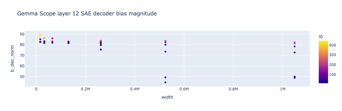
We see the general trend that decoder bias decreases as the SAE gets wider. However, there also appears to be a correlation between L0 and the decoder bias norm, with lower L0 SAEs having a much lower decoder bias norm, especially at higher widths. The delta between the largest and smallest decoder bias norms seen here is especially large, nearly doubling from the lowest to highest decoder bias norm. We do not have a good explanation as to why there should be a correlation between L0 and decoder bias norm.
Discussion
Feature hedging is likely a serious problem in existing LLM SAEs, and may help explain why recent results have found SAEs consistently underperform on probing and steering. We should expect hedging to occur any time an SAE is narrower than the number of “true features”, and these features have any correlation at all with features tracked by the SAE. Hedging will cause SAE latents to merge in positive and negative components of all correlated external features, and this will likely cause the SAE latents to both underperform as classifiers and break the model when used as steering vectors.
We presented a novel reconstruction loss, snap loss, which solves hedging in toy models if the magnitude of the hedging is low, but fails to solve hedging if the magnitude of the hedging is high. Empirically, we find that snap loss does not seem to be obviously helpful in LLM SAEs, so this may be evidence that the level of hedging in LLM SAEs is high, or that snap loss is not useful in reality. We also show signs that hedging occurs in SAEs trained on LLM activations by tracking changes to existing latents as new latents are added. However, we still do not have a metric that can be easily calculated on a given SAE to determine the level of hedging in SAE activations without growing the SAE, which makes designing architectures around solving hedging challenging. We are also uncertain about how to interpret the SAE decoder bias norm, and whether there is an easily identifiable link between the decoder bias norm and the amount of hedging in an SAE.
Citation (please cite the paper)